1. Introduction
According to the sixth assessment report released by the United Nations Intergovernmental Panel on Climate Change (IPCC) in 2021, the Earth’s global average surface temperature rose by approximately 1.09 °C compared to the level between 1850 and 1900 [
1]. It is estimated that unless carbon dioxide and other greenhouse gas emissions are significantly reduced in the coming decades, global warming will exceed 1.5 °C or even 2 °C by the end of the 21st century [
2,
3]. Global warming has disturbed the balance of the Earth’s radiation budget (ERB). As a result, extreme weather events (such as dust storms, heat waves, tropical cyclones, severe convection, and droughts in some regions) will occur with increasing frequency [
4,
5,
6]. Accurate measurements of the ERB can help us to understand the Earth’s radiation imbalance [
7]. The causes of weather and climate change and the feedback of extreme weather and greenhouse gases will also be discussed in depth.
Instrument design and calibration determine the accuracy of the integrated ERB. Currently, global radiation is measured by scanning the Earth with polar satellites equipped with narrow field of view (NFOV) radiometers [
8,
9]. By improving the scanning accuracy and fitting the scanning data of different time series perfectly, one can obtain detailed information on the integrated ERB. NASA’s Cloud and Earth Radiant System (CERES) scans the Earth on a 20 km spatial scale [
10,
11]. It is the system with the longest observation history and the highest measurement accuracy in recent years. CERES aims to measure outgoing longwave radiation (OLR) with an accuracy of 0.5% and reflected solar radiation with an accuracy of 1% for decades to understand the diversity of natural climate variability [
12,
13]. Moreover, the in-flight calibration of CERES completely depends on the internal calibration systems [
14,
15]; the degradation of the instrument cannot be directly measured during long-term observation. The observation accuracy poses a great challenge to on-orbit monitoring. Consequently, CERES plans to correct uncertainties caused by instrument aging based on lunar scanning data from NASA’s Lunar and ERB Experiment (MERBE) mission [
16]. Another NASA program, CubEshine, plans to observe the intensity of earthshine on the Moon that can be used to constrain terrestrial shortwave albedo in the hemispheric-average sense [
17]. The broadband bolometric oscillation sensor (BOS) operates as part of the payload of the PICARD microsatellite, which adopted a new method that estimates the global net radiation at the TOA based on the satellite measurements [
18].
We aim to develop a staring radiometer to collect global ERB. It will perform ERB observation and lunar radiometric calibration at the Lagrange L1 point of the Earth–Moon system. At point L1, any object maintains its relative position to the Earth and the Moon [
19]. The position and attitude of the lunar centroid in the coordinate system are fixed, and the nearside of the Moon always faces the Earth and the L1 point [
20]. The integral Earth radiation at the hemispheric spatial scale can be obtained directly using our radiometer, and global radiation can be collected in a matter of hours. In addition, the Moon will be used as a stable source combined with internal sources for in-flight calibration to ensure the accuracy of long-term ERB observations. Lunar scanning data from different payloads, such as CERES, will no longer be required. Through the direct observation of the lunar integral radiation, the aging of the radiometer can be corrected.
This manuscript presents the observation system of the radiometer including the design of an optical system, the analysis, and the suppression of stray radiation. Since our radiometer carries out radiation observations at point L1 of the Earth–Moon system, the Earth’s radiation signal is weak, and the influence of stray light on the observation must be minimized; therefore, this manuscript not only studies the optical system of observation but also focuses on the sources of internal and external stray radiation and elimination methods of the system so as to realize the observation ability of the radiometer. In this paper, the telescope adopts the Cassegrain system and uses the combination of two-stage baffle, inner baffle, and inclined vertical vanes to eliminate the external stray radiation and temperature compensation to eliminate the influence of thermal stray radiation on the observation. The paper is structured as follows:
Section 2 introduces the instrument design concept;
Section 3 highlights the optical design constraints, optical design, and image quality analysis of the optical system;
Section 4 describes the stray radiation sources and suppression methods; the simulation results of the radiometer’s stray radiation and the verification of the suppression ability are given in
Section 5;
Section 6 discusses our findings; finally, the conclusions are presented in
Section 7.
2. Instrument Design Concept
An orbiter will carry a non-scanning radiometer package for ERB observation and lunar radiation calibration at point L1 as shown in
Figure 1. The radiometer is equipped with two channels: one is a total wavelength (TW) channel, measuring Earth reflected and emitted radiation in the 0.2–50.0 μm spectral range; the other is a short wavelength (SW) channel that measures Earth’s reflected radiation in the 0.2–5.0 μm spectral region. Each channel contains a Cassegrain telescope. In the SW channel, a low-pass filter is placed in front of the detector to filter out the longwave radiation. A two-stage fore baffle and an inner baffle are used in each channel to eliminate stray radiation. TW and SW data are sampled by the thermoelectric detector and electronic systems.
The design of the radiometer’s observation system is limited by the launch conditions, and many factors need to be considered to ensure that it meets the use requirements while remaining a compact structure. At the same time, the altitude of the orbiter is up to 3.27 × 10⁵ km, so the measured TW and SW are weak. As the Earth and the Moon rotate around the sun, the ERB detected by the system runs the risk of being embedded in strong solar radiation and cannot be identified. During radiation detection, the temperature increase of the system’s components will bring thermal radiation, which is also the main source of stray radiation. Therefore, the analysis and suppression methods of stray radiation are particularly important.
3. Optical System
3.1. Constraints of Optical System
To determine the optical system parameters, we analyzed the observing geometry. As shown in
Figure 2, the field of view (FOV) angle of the telescope 2ω should satisfy Equation (1).
where
is half the FOV angle for observation of the Earth’s hemisphere at point L1;
is half the FOV angle for observation of the lunar hemisphere at point L1. The
and
are given by Equation (2):
where
,
is the Earth’s radius, where
= 6371 km;
is the distance between the Earth’s centroid and point L1. Similarly,
,
is the lunar radius, where
= 1737.1 km;
is the distance between the lunar centroid and point L1.
According to the position feature of L1,
and
can be expressed as the Earth–Moon distance, that is:
where
d is the average Earth–Moon distance (
d = 384,403.9 km).
The diameter
of the detector used in the radiometer is 4 mm. Equation (4) should be satisfied to constrain the half image height (
h) and maintain complete imaging of the Earth and Moon by the detector.
3.2. Optical Design
Our radiometer is used for the measurement of wide-spectrum Earth integral radiation, which is mainly used in the study of the Earth’s radiation budget (ERB). For our thermal radiation detection system, the telescope operates in the spectral region from 0.2 to 50.0 μm. Reflective optical systems, rather than transmissive optical systems, are necessary to avoid severe chromatic aberration. Due to the fact that our radiometer does not have high requirements for resolution, we adopted a two-mirror telescope in order to control the volume and quality of the system. The Cassegrain system satisfies all observation demands and uses a single detector to receive radiation. Apart from this, the system is more compact and convenient for processing and alignment than an off-axis telescope. Thus, a Cassegrain system is the most suitable telescope for our radiometer. To detect weak Earth radiances, the aperture of the optical system should not be too small. It was preliminarily determined that the ERB can be fully measured when the aperture is 40 mm through radiant flux estimation. The aperture was determined by comprehensively considering the Earth’s radiation flux measured by the detector and launch conditions of the radiometer. Equations (5)–(12) in the manuscript are the methods of radiation power calculation. If the aperture of our telescope is too large, the volume and mass of the baffle will increase accordingly. If the aperture is too small, the observed Earth radiation power will be too weak. This is an iterative process to ensure the radiometer’s Earth radiation observation ability. The volume and mass of the radiometer should not be too large in order to save launch resources. The manuscript presents the optimal results after the design and calculations with different telescope diameters. According to the analysis in the previous section, the design indexes of the optical system become clear as shown in
Table 1. Parameters of the optics are defined according to the theoretical design, and then optimized by ZEMAX, which is a widely used optical system design and optimization software.
Two shaded models of the optimized optical systems output in ZEMAX are shown in
Figure 3. The optical system in each channel contains two mirrors: one primary mirror adopts a paraboloid surface, and one secondary mirror adopts a hyperboloid surface. The telescopes have no spherical aberrations and are convenient to manufacture [
21]. It should be noted that the mirrors in both channels are the same. Nevertheless, the SW channel contains a low-pass filter; thus, the back working distance of the optical system in the two channels are different. For the Cassegrain system, the 4° full field of view is too large to control the obstruction ratio at a small value when meeting the image height requirements. Additionally, the system does not include refractive optics, and there are fewer variables that can be optimized. Therefore, taking the curvature radius, conic coefficient, and separation of the two mirrors as the optimization variables, the image height was controlled within 4 mm, and the obstruction rate was expanded to 0.51. The final telescope is a f/1.13 Cassegrain that has a 40 mm diameter aluminized primary mirror and an aluminized secondary mirror. The conic coefficient of the primary mirror is −1, and that of the secondary mirror is −5.556. The primary and secondary mirrors are placed 10 mm apart. Respectively, the back working distance of the optical system in the TW channel and SW channel is 8 and 3 mm, respectively. The structural parameters of the telescope are shown in
Table 2.
3.3. Optical System Performance
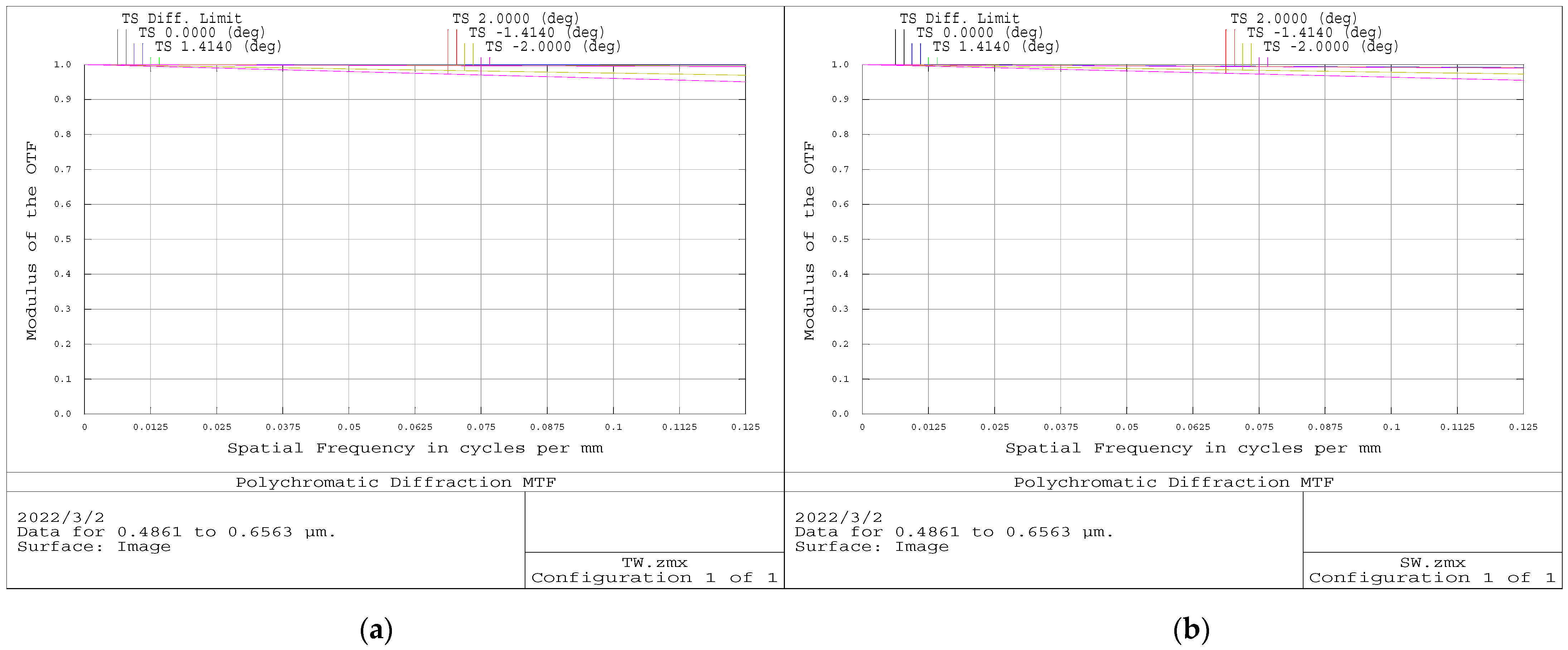
The modulation transfer function (MTF) was applied to evaluate the imaging quality. Meanwhile, the spot diagram and footprint diagram were analyzed.
Figure 4 shows the MTF curves of the optical systems in the TW and SW channels. At the Nyquist frequency of 0.125 cycles/mm (which is defined as 0.5 cycles per pixel) [
22], the MTF values were close to the diffraction limit.
As can be seen from the spot diagrams in
Figure 5, the RMS of the optical system in the TW channel was 143.228 μm, and the other was 131.522 μm. Although the image discs were larger than airy discs, according to the footprint diagrams in
Figure 6, the full-field images were located in the receiving surface of the detector. The image height of each FOV was less than 4 mm, and the aberration in the optical system was within the acceptable range. The optical systems thus have good imaging quality.
4. Stray Radiation Suppression
4.1. Stray Radiation Suppression Requirement
When the Earth and Moon rotate around the Sun, the sunlight will directly irradiate the telescope at an angle to the telescope’s optical axis, which will not happen only when the Sun is blocked by the Earth. During observation, the sunlight will bring strong stray radiation, also known as stray light. Thus, we plan to eliminate the stray radiation when the Sun is at least 45° off the optical axis. We considered that when the solar incident radiation is suppressed to 0.01% of the ERB radiation collected by the detector, the effect of external stray radiation on measurement can be ignored. Point source transmittance (PST) was adopted to evaluate the suppression level of the observation system, which is defined as the ratio of the irradiance generated by the external field source on the image surface to the irradiance at the entrance port [
23]. The requirements of stray radiation suppression were analyzed before designing the suppression structure.
Taking the Sun as a black body with a temperature of
Tsun = 5900 K [
24], the solar irradiance in the spectral range of 0.2–5.0 μm is given by:
where
is the wavelength, and
and
are the black body radiation constants.
Solar radiation intensity
can be written as:
where
is the radius of the Sun.
The solar irradiance at the entrance pupil of the radiometer is given by:
where
is the angle between the Sun and the optical axis, and
l is the distance between the optical system and the Sun, approximately the distance between the Sun and the Earth.
Considering the Earth as a gray body with a temperature,
= 288 K, and a bond albedo
= 0.3 [
25,
26], the Earth’s radiance in the spectral range of 0.2–50 μm can be described as:
The Earth’s radiant radiance,
, in the 5.0–50.0 μm spectral region is:
The Earth’s reflected radiance in the 0.2–5.0 μm spectral region is given by:
In
, the solar irradiance on Earth
can be calculated as:
where
is the view angle of the Sun to the Earth.
The Earth’s radiant power received by the detector,
, is given by:
where
is the surface reflectance of the primary and secondary mirrors,
is the effective utilization area of the mirror except obstruction, and
is the half FOV angle applied for the observation of the Earth.
The value of the Earth’s irradiance received by the detector,
, can be obtained from the formula:
The PST of the system should satisfy Equation (14):
Parameters in the appeal inequality are shown in
Table 3. Finally, the PST at the 45° off-axis angle should satisfy Equation (15):
4.2. Stray Radiation Suppression Structure Design
4.2.1. Two-Stage Outer Baffle Design
The system requires high PST, and the space available for extinction structures between the primary and secondary mirrors is limited. Setting light trapping in the mirrors’ barrel makes little contribution to the stray light suppression, so a two-stage outer baffle was designed to eliminate the main external stray light. The structural parameters of the baffle were determined by the off-axis angle
and the telescope’s FOV and effective aperture. The length and aperture of the baffle is given in Equation (16):
where
i is the number of stages of the baffle;
Di−1 is the diameter of the
i-th stage baffle’s light inlet;
Di is the diameter of the
i-th stage baffle’s light outlet;
Li is the length of the
i-th stage baffle.
The baffle cannot block the available imaging light [
27]. Since not only the telescope but also the mirrors’ barrel and other structural elements are mounted behind the baffle, the baffle’s aperture must be larger than the telescope’s entrance pupil. However, the size of the baffle should not be too large to avoid increasing the volume and weight of the radiometer. The design parameters of the two-stage baffle in this paper are shown in
Table 4.
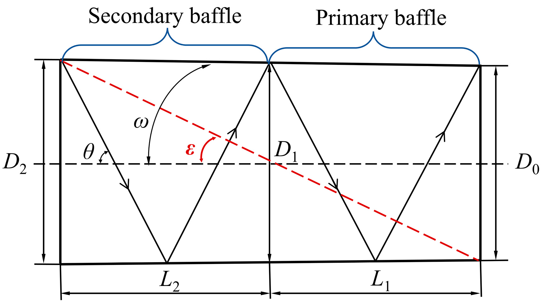
Figure 7 shows the design principle of the baffle. It can be seen from the figure that the stray radiation suppression capacity of the two-stage hood is higher than that of the one-stage hood. Our two-stage baffle can suppress stray radiation with an off-axis angle greater than
(
= 15°). When the angle between stray light and the optical axis is less than 15°, it can directly enter the optical system without reflection. Other off-axis incident rays are reflected in our baffle at least four times before reaching the telescope.
To achieve the required stray radiation suppression capability, the baffle alone is not enough. Several vanes are designed inside the baffle to form light trappings to increase the reflection of stray light. In addition, a layer of black paint with high absorption efficiency, named Nextel level coating 811-21, is coated on the inner surface of the baffle, the vanes, and the mechanical components to suppress stray light effectively.
According to the design principle of the vanes, the stray light irradiated inside the baffle cannot directly enter the optical system after one scattering, and the vanes cannot block the FOV [
28]. Thus, a certain length is extended for each vane outside the baffle. On the basis of the baffle vanes’ geometrography method [
29], the light inlet of the baffle is taken as the first vane, and the intersection of the connection line between the bottom end and the top of the baffle’s light outlet and FOV of the optical system can determine the position and height of the second vane. Therefore, the position of all the vanes can be obtained. As a result, both the primary and second baffle contain seven non-equidistant vanes in our two-stage baffle. From our research on the vanes, we know that when there is a certain inclination between the vanes and the inner wall of the baffle, its suppression ability is better than that of vertical vanes [
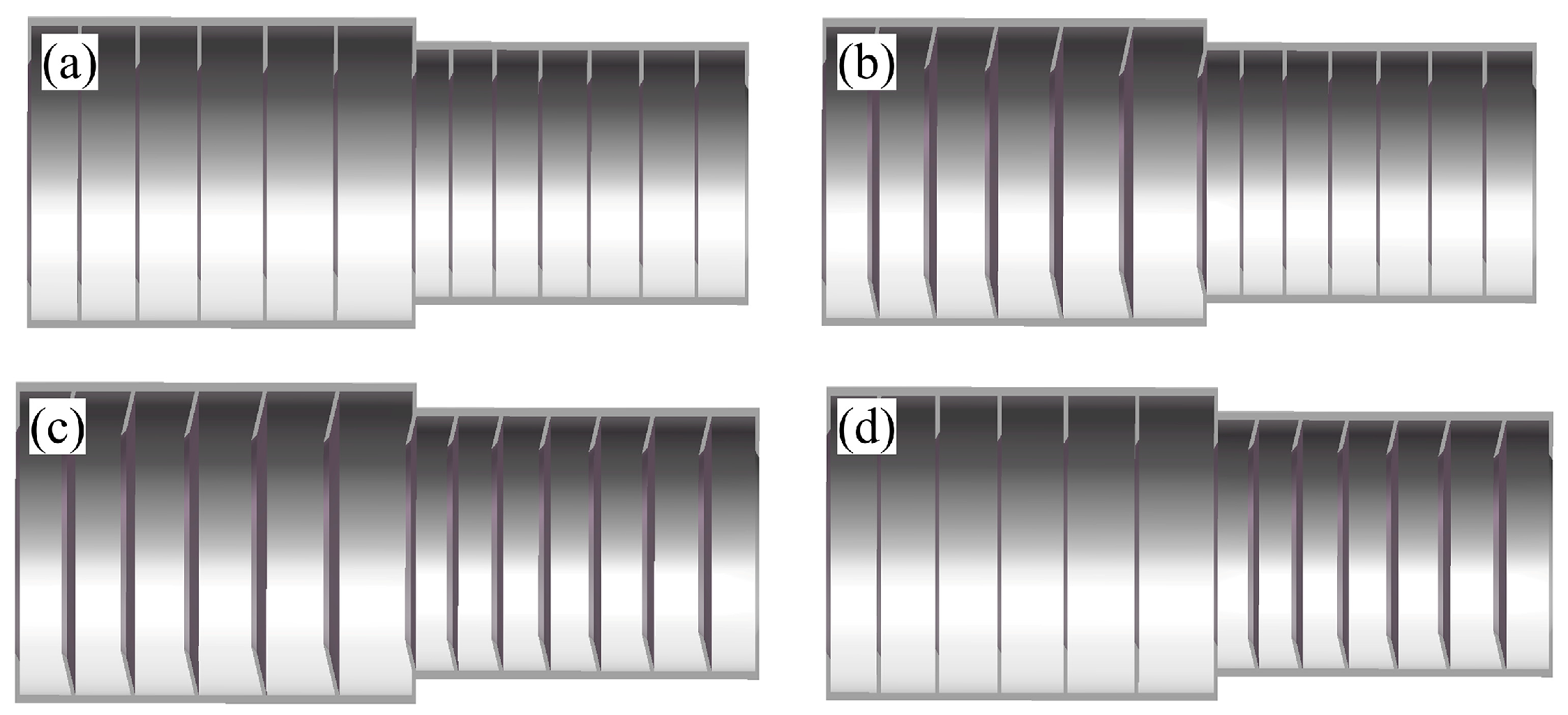
30]. According to the different distribution of the vertical or inclined vanes in the two-stage baffle, four structures were designed as shown in
Figure 8. All vanes in structure (a) are vertical to the inner wall of the baffle. In structure (b), the vanes in the primary baffle are vertical, and the vanes in the second baffle are inclined at 77°. All vanes in structure (c) are inclined at 77°. Additionally, in structure (d), the vanes in the primary baffle are inclined at 77°, the others are vertical. In
Section 5, the stray light suppression capacity of the four structures are compared and analyzed to select the best one.
4.2.2. Inner Baffle Design
Figure 9 shows the design method of the inner baffle. The front aperture diameter MM’ was determined by the intersection of the edge-rays reflected by the mirrors, and the aperture of the baffle resting on the primary mirror should be equal to or less than the aperture SS’, which was determined by the intersection of the marginal ray passing through the edge of the front aperture and the primary mirror [
31]. The light outlet diameter NN’ of our inner baffle is the same as the primary mirror hole diameter. The inner baffle can not only eliminate the external stray radiation but also limit the FOV of the detector and reduce the thermal radiation detected by the system.
5. Stray Radiation Analysis
5.1. External Stray Radiation Analysis
5.1.1. Simulation Setting
After establishing the three-dimensional model of the observation system, the stray light suppression performance was simulated by ray tracing based on the Monte Carlo method [
32]. We simplified the mechanical structure when tracing rays by retaining the main structural elements and removing small parts such as screws. The explosion diagram of the simulation model is shown in
Figure 10, in which the TW channel does not contain the filter. The position of the simulated circular grid sources completely coincided with the entrance pupil of the baffle. By setting the ray direction vector to adjust the angle between the light beam and the optical axis, the sunlight entering the optical system at an off-axis angle of 0–80° was simulated. Each light beam contained 7.6 million rays.
5.1.2. Surface Properties
Before simulation, it was necessary to set the optical properties of all component surfaces such as specular reflection, scattering, and transmission. Bidirectional reflection distribution function (BRDF) is a common method used to describe the scattering characteristic of a surface [
33]. An optical simulation software development company named Lambda Research Corporation is equipped with special precision instruments to measure the scattering characteristics of different materials. The optical elements and the detector used the calculated model from this company [
34]. Other surfaces were coated with NEXTEL Velvet Coating 811-21, and its model is given in the official data from the company and several test results [
35,
36]. In the simulation, we believe that the absorptivity of the coating under actual working conditions may attenuate and make it lower.
Table 5 shows the surface property parameters.
5.1.3. Simulating External Stray Radiation
The four structures of the TW channel designed in
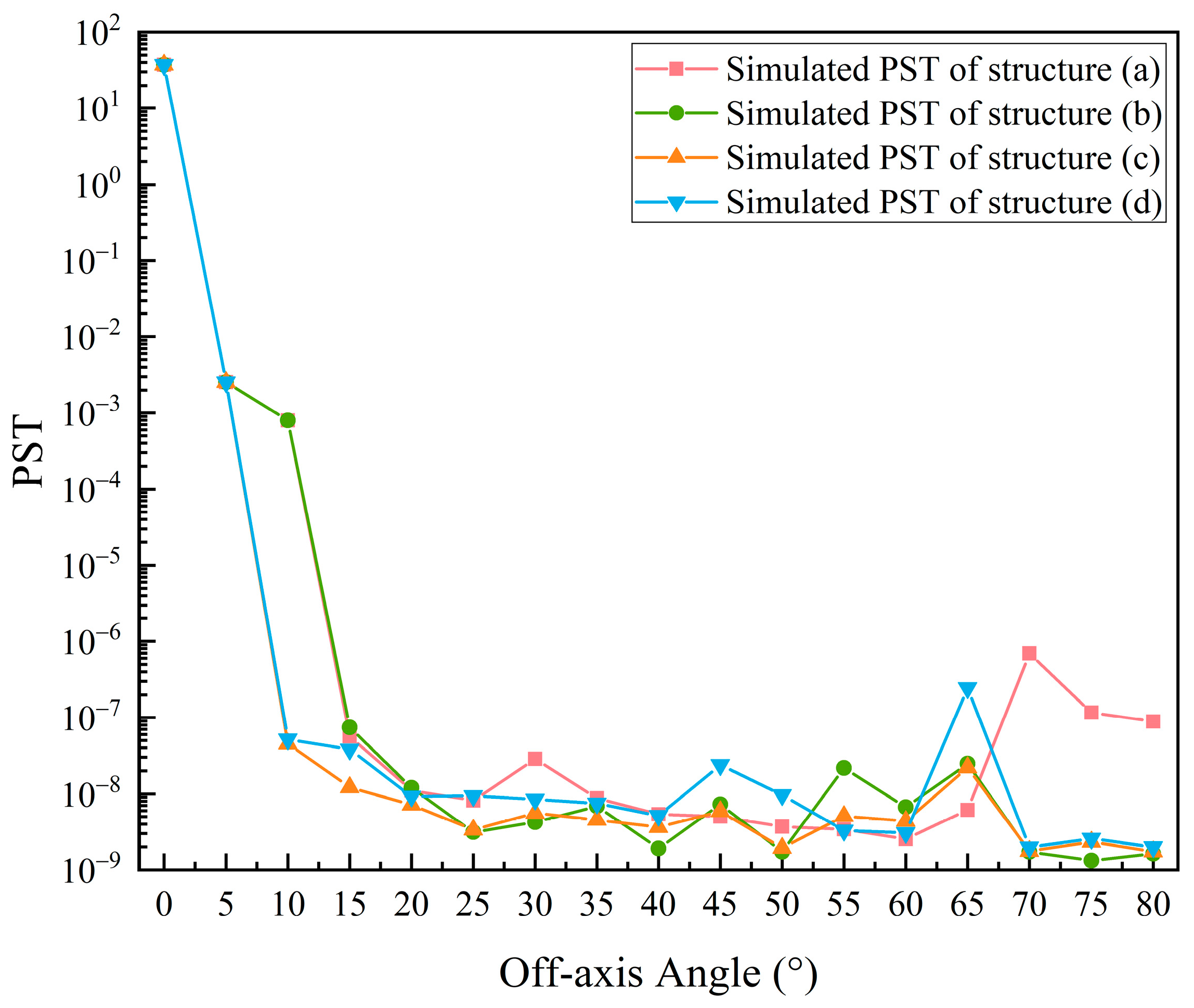
Section 4.2. were assembled with the optics and mechanics used for simulation through Monte Carlo ray tracing. Under the same setting conditions, the simulation was performed at an interval of 5°. Finally, the PST curves of the four structures were obtained when the off-axis angle is 0–80° as represented in
Figure 11 below. It can be seen from the results that for the extinction ability of stray light, structure (c) was the best. It was thus adopted for our radiometer.
Structure (c) was then assembled in the SW channel and simulated.
Table 6 shows the main stray light ray paths of the two channels when the off-axis angle was 45°. Obviously, the baffles played a great role in the stray light suppression. Additionally, the critical surfaces in the ray paths of the system were coated with black paint with high absorptivity apart from optics. The stray light entering the system was reflected and absorbed many times inside the telescope.
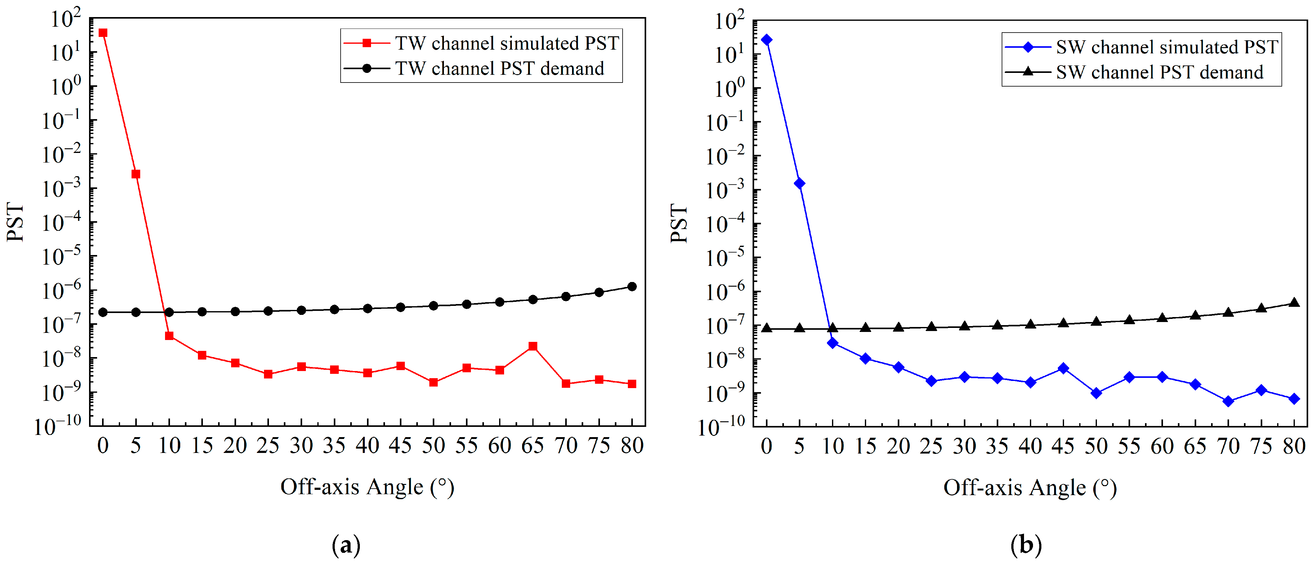
Figure 12 shows the simulation PST and required PST curves of the two channels. Both channels had a good ability to suppress external stray radiation, which was much better than the theoretical required value at the corresponding angle. The radiometer can start to measure ERB when the solar off-axis angle is 10°, and the external stray radiation can be ignored during observation. The observation time of the radiometer was longer than the expected target observed outside the 45° solar off-axis angle.
5.2. Internal Stray Radiation Analysis
High absorptivity means high emissivity. In order to suppress external stray radiation, the absorptivity of the inner surface coating was as high as 0.95. An increase in system temperature will bring additional internal stray radiation, that is, thermal radiation from the components.
5.2.1. Internal Stray Radiation Source
Since the light path is reversible, the surface irradiated on the detector is also the visible surface of the detector. To find the thermal radiation sources, we set the detector as a Lambertian source with a certain radiant flux and then performed reverse ray tracing based on the Monte Carlo method. The radiant flux received by each component of the system is analyzed through the simulation results. Surfaces that receive more energy emit more thermal radiation. The energy received by the components as a percentage of the total radiant flux is shown in
Figure 13.
In the TW channel, 99.194% of thermal radiation came from the spider, mirrors, inner baffle, and end cover. In the SW channel, 99.638% of thermal radiation came from the spider, mirrors, inner baffle, filter, and end cover. Additionally, thermal radiation from the detector gland could not be detected in either channel.
5.2.2. Simulating Internal Stray Radiation
Although the sources of internal stray radiation were found, it was necessary to quantitatively analyze the stray radiation because of the different properties of the surface coating. The contribution of different components to stray radiation were analyzed. The detector was set as a black body, the other elements in the system were set as gray bodies, and their emissivity was the same as the absorptivity given in
Table 5. A simulation was run every 10 K between 100 and 350 K for each element.
Figure 14 and
Figure 15 show the results.
In the SW channel, the presence of a filter greatly weakened the infrared thermal stray radiation of many components. However, the thermal radiation of the components located behind the filter was not greatly attenuated. Additionally, the radiometer will work at room temperature instead of at a low temperature. In order to completely remove internal thermal radiation, it is necessary to control the entire machine in a low-temperature environment. This requires huge refrigeration equipment, and the mirrors are at risk of deformation, resulting in defocusing and other phenomena. Therefore, we plan to take the thermal radiation as a stable background noise through temperature control, remove it by setting a compensation detection unit, and cooperate with the weak signal measurement system to collect the TW and SW radiation.
5.2.3. Error Budget
Table 7 and
Table 8 show the irradiance values and error budgets of the system at 100, 293.15, and 300 K. We simulated the element thermal irradiance error in the two channels when the temperature was perturbed by ±0.1 K and calculated the corresponding synthesized error budget. The values of 100 and 350 K show that the thermal radiation suppression requirement of the system at extremely low temperatures was lower than that at high temperatures and that the system needs to choose an appropriate operating temperature and accurate temperature control.
6. Discussion
An ERB radiometer based on the L1 point of the Earth–Moon system was proposed in this paper. A two-channel radiometer using a shared Cassegrain telescope and a low-pass filter can achieve TW and SW measurements in the spectral range of 0.2–5.0 μm and 0.2–50.0 μm, respectively. Each channel had a two-stage outer baffle and an inner baffle to eliminate stray radiation. ERB was collected by a thermoelectric detector. A major weakness of previous ERB radiometers is the indirect measurement of radiation. The integral ERB was obtained by scanning data fitting. Our radiometer can make up for this deficiency. Global radiation is obtained from multiple hemispherical integral radiation observations over several hours based on the rotation of the Earth. The Earth’s mean radiation budget is measured over a short time series. At the same time, the direct observation of lunar radiation is a method of in-flight calibration. The next step will be the realization of this radiometer.
Some problems need to be considered during the radiometer design. Initially, the system needs to be able to observe the hemispheres of the Earth and the Moon. To solve this issue, we analyzed the requirements of the FOV for optical systems. It was found that the radiometer required high image quality in the FOV of 4°, which was implemented by increasing the obstruction ratio to 0.51 of the Cassegrain telescopes during optimization. After that, the sunlight and thermal radiation of the optical system would interfere with the measurement. Thus, we analyzed the stray light suppression requirements of the system at different solar off-axis angles. To suppress sunlight beyond the 45° off-axis angle, we designed a two-stage baffle. Four structures were designed according to the distribution of vertical and inclined vanes in the baffle to improve PST. The simulation results indicated that the suppressing of stray light ability was the best when the vanes were all inclined at 77°. The PST of each channel showed that the radiometer could start observing at a 10° off-axis angle. The ability of the system to eliminate external stray radiation could reach the order of 10−8. Stray light path analysis indicated that the use of baffles and black paint had great stray light suppression ability. Due to the limited capabilities of the simulation software, the PST curve fluctuated at some angles, but, overall, the capability of the proposed system to cancel the stray light effect was far better than required. Beyond that, the variation of black paint absorptivity with spectrum and the attenuation of instrument in orbit measurement were not considered in the simulation. During instrument observation, it was necessary to actually measure and correct the absorption attenuation of the coating.
In addition, it was also important to analyze internal stray radiation. A preliminary analysis showed that all elements in the telescopes were internal stray radiation sources except for the detector gland through reverse ray tracing. The detector gland was not visible to the detector receiving surface and its thermal radiation could not be measured. Other surfaces visible to the detector would affect the measurement as the temperature increased, which would depend on temperature changes and the emissivity of the surfaces. Then, we performed thermal irradiance for each element on the detector at temperatures ranging from 100 to 350 K. The thermal radiation curves of all components received by the detector had the same variation trend in the TW channel. In the SW channel, longwave infrared radiances of the front components were filtered out due to the presence of the filter. However, the components behind the filter were still inevitably irradiated to the detector, so the irradiance curves of the filter, end cap, detector, and detector gland were different from the other elements. The results show that the internal stray radiation had little impact on the observation when the system was at a low temperature (~100 K) but could not be ignored when the temperature increased. From the system error budget analysis, once the radiometer is used at a temperature of 293.15 K, the thermal radiation temperature of the system should be well controlled and using it at a high temperature should be avoided.
Through the design of the optical system and the analysis and elimination of the stray radiation of the system, our radiometer has a practical radiation observation performance at the L1 point of the Earth–Moon system.
7. Conclusions
We proposed a new ERB radiometer based on an optimized optical design and a stray radiation simulation. The radiometer has two channels to observe Earth’s reflected solar radiation and reemitted OLR radiation. Radiometers observe radiation through a Cassegrain telescope and receive radiation through a thermoelectric detector. The telescope has good imaging quality. An assessment of the image quality was conducted by characterizing the MTF, spot diagram, and footprint diagram. The MTF of two telescopes were close to the diffraction limit at 0.125 cycles per mm and full-field image heights were less than 4 mm. Two-stage outer and inner baffles were designed to suppress external stray radiation and to limit the FOV of the detector. The ray path analysis and stray light simulation results showed that stray radiation was effectively suppressed, and when the solar off-axis angle was 10°, the PST of each channel reached the order of 10−8. External stray radiation can be suppressed to 0.01% of the valid ERB. The Irradiance curve and error budget of each internal stray radiation source from 100 to 350 K were subsequently analyzed. We plan to eliminate the inner thermal radiation as background radiation through temperature control and compensation. Reasonable temperature control and correction are challenging but not impossible and will be further optimized in subsequent prototype development. All analyses showed that our observation system has reliable ERB measurement performance at the L1 point. Integrated ERB can be observed, and the Moon will be used as a stable natural calibration source for on-orbit calibration. Thus, the instrument aging error is monitored and corrected over time.
In addition to the scientific objectives of this paper, working out how to obtain more detailed ERB information using the observation data of scanning radiometers is a potential direction for further research.
Author Contributions
Conceptualization, X.Y., P.Z. and W.F.; methodology, H.Z. and X.Y.; software, H.Z. and Y.W.; validation, H.Z., X.Y., P.Z. and Y.W.; formal analysis, H.Z., X.Y. and P.Z.; investigation, H.Z., P.Z. and X.Y.; resources, X.Y. and P.Z.; data curation, H.Z.; writing—original draft preparation, H.Z., P.Z. and X.Y.; writing—review and editing, H.Z., P.Z. and X.Y.; visualization, H.Z.; supervision, X.Y. and P.Z.; project administration, X.Y., P.Z. and W.F.; funding acquisition, X.Y. All authors have read and agreed to the published version of the manuscript.
Funding
This research was funded by the National Key Research and Development Program of China (No. 2018YFB0504600 and 2018YFB0504603).
Data Availability Statement
Not applicable.
Acknowledgments
This work was partly supported by the National Science Foundation of China (Grant Number: 41974207). This work was also supported by the Moonbase exploration research equipment purchase project of the Development and Reform Commission of Shenzhen Municipality (No. 2106-440300-04-03-901272).
Conflicts of Interest
The authors declare no conflict of interest.
Abbreviations
The following abbreviations are used in this manuscript:
| ERB | Earth’s radiation budget |
| TOP | Top of the atmosphere |
| IPCC | Intergovernmental Panel on Climate Change |
| NFOV | Narrow field of view |
| CERES | Cloud and Earth Radiant System |
| OLR | Outgoing longwave radiation |
| MERBE | Lunar and ERB Experiment |
| BOS | Bolometric oscillation sensor |
| TW | Total wavelength |
| SW | Short wavelength |
| FOV | Field of view |
| EPD | Entrance Pupil Diameter |
| EFL | Effective Focal Length |
| MTF | Modulation transfer function |
| RMS | Root mean square |
| PST | Point source transmittance |
| BRDF | Bidirectional reflection distribution function |
References
- Arias, P.; Bellouin, N.; Coppola, E.; Jones, R.; Krinner, G.; Marotzke, J.; Naik, V.; Palmer, M.; Plattner, G.-K.; Rogelj, J.; et al. Technical Summary. In Climate Change 2021: The Physical Science Basis. Contribution of Working Group I to the Sixth Assessment Report of the Intergovernmental Panel on Climate Change; Cambridge University Press: Cambridge, UK, 2021. [Google Scholar]
- Chen, D.; Lai, H.-W. Interpretation of the IPCC AR6 WGI report in terms of its context, structure, and methods. Adv. Clim. Change Res. 2021, 17, 636. [Google Scholar]
- Cai, W.; Ng, B.; Wang, G.; Santoso, A.; Wu, L.; Yang, K. Increased ENSO sea surface temperature variability under four IPCC emission scenarios. Nat. Clim. Change 2022, 12, 228–231. [Google Scholar] [CrossRef]
- Wasko, C. Can temperature be used to inform changes to flood extremes with global warming? Philos. Trans. R. Soc. A 2021, 379, 20190551. [Google Scholar] [CrossRef] [PubMed]
- Geiger, T.; Gütschow, J.; Bresch, D.N.; Emanuel, K.; Frieler, K. Double benefit of limiting global warming for tropical cyclone exposure. Nat. Clim. Change 2021, 11, 861–866. [Google Scholar] [CrossRef]
- Shi, L.; Zhang, J.; Yao, F.; Zhang, D.; Guo, H. Drivers to dust emissions over dust belt from 1980 to 2018 and their variation in two global warming phases. Sci. Total Environ. 2021, 767, 144860. [Google Scholar] [CrossRef]
- Dewitte, S.; Clerbaux, N.; Cornelis, J. Decadal changes of the reflected solar radiation and the earth energy imbalance. Remote Sens. 2019, 11, 663. [Google Scholar] [CrossRef] [Green Version]
- Dewitte, S.; Clerbaux, N. Measurement of the Earth radiation budget at the top of the atmosphere—A review. Remote Sens. 2017, 9, 1143. [Google Scholar] [CrossRef] [Green Version]
- Gristey, J.J.; Su, W.; Loeb, N.G.; Vonder Haar, T.H.; Tornow, F.; Schmidt, S.K.; Hakuba, M.Z.; Pilewskie, P.; Russell, J. Shortwave Radiance to Irradiance Conversion for Earth Radiation Budget Satellite Observations: A Review. Remote Sens. 2021, 13, 2640. [Google Scholar] [CrossRef]
- Loeb, N.G.; Kato, S.; Loukachine, K.; Manalo-Smith, N.; Doelling, D.; Technology, O. Angular distribution models for top-of-atmosphere radiative flux estimation from the Clouds and the Earth’s Radiant Energy System instrument on the Terra satellite. Part II: Validation. J. Atmos. Ocean. Technol. 2007, 24, 564–584. [Google Scholar] [CrossRef]
- Smith, G.; Priestley, K.; Loeb, N.; Wielicki, B.; Charlock, T.; Minnis, P.; Doelling, D.; Rutan, D. Clouds and Earth Radiant Energy System (CERES), a review: Past, present and future. Adv. Space Res. 2011, 48, 254–263. [Google Scholar] [CrossRef]
- Priestley, K.J.; Smith, G.L.; Thomas, S.; Cooper, D.; Lee, R.B.; Walikainen, D.; Hess, P.; Szewczyk, Z.P.; Wilson, R.; Technology, O. Radiometric performance of the CERES Earth radiation budget climate record sensors on the EOS Aqua and Terra spacecraft through April 2007. J. Atmos. Ocean. Technol. 2011, 28, 3–21. [Google Scholar] [CrossRef]
- Rose, F.G.; Rutan, D.A.; Charlock, T.; Smith, G.L.; Kato, S.; Technology, O. An algorithm for the constraining of radiative transfer calculations to CERES-observed broadband top-of-atmosphere irradiance. J. Atmos. Ocean. Technol. 2013, 30, 1091–1106. [Google Scholar] [CrossRef]
- Folkman, M.A.; Jarecke, P.J.; Hedman, T.R.; Yun, J.S.; Lee, R.B., III. Design of a solar diffuser for on-orbit calibration of the Clouds and the Earth’s Radiant Energy System (CERES) instruments. In Proceedings of the Sensor Systems for the Early Earth Observing System Platforms, Orlando, FL, USA, 25 August 1993; Volume 1939, pp. 72–81. [Google Scholar]
- Lee, R.B., III; Barkstrom, B.R.; Smith, G.L.; Cooper, J.E.; Kopia, L.P.; Lawrence, R.W.; Thomas, S.; Pandey, D.K.; Crommelynck, D.; Technology, O. The Clouds and the Earth’s Radiant Energy System (CERES) sensors and preflight calibration plans. J. Atmos. Ocean. Technol. 1996, 13, 300–313. [Google Scholar] [CrossRef]
- Matthews, G. NASA CERES Spurious Calibration Drifts Corrected by Lunar Scans to Show the Sun Is not Increasing Global Warming and Allow Immediate CRF Detection. Geophys. Res. Lett. 2021, 48, e2021GL092994. [Google Scholar] [CrossRef]
- Thejll, P.; Barjatya, A.; von Hippel, T.; Lukashin, C.; Gleisner, H.; Flynn, C. CubEshine: A cube-sat project for earthshine observations of the Moon. In Proceedings of the EGU General Assembly Conference Abstracts, Vienna, Austria, 4–13 April 2018; p. 6119. [Google Scholar]
- Zhu, P.; Wild, M.; Van Ruymbeke, M.; Thuillier, G.; Meftah, M.; Karatekin, O. Interannual variation of global net radiation flux as measured from space. J. Geophys. Res. Atmos. 2016, 121, 6877–6891. [Google Scholar] [CrossRef] [Green Version]
- Salazar, F.; Macau, E.E.; Winter, O.C. Chaotic dynamics in a low-energy transfer strategy to the equilateral equilibrium points in the Earth–Moon system. Int. J. Bifurc. Chaos 2015, 25, 1550077. [Google Scholar] [CrossRef]
- Li, H. Communicating with lunar orbiter by relay satellites at earth-moon lagrange points. In Proceedings of the International Conference on Advanced Computer Science and Electronics Information, Beijing, China, 25–26 July 2013; pp. 418–422. [Google Scholar]
- Jie, L.; Jingqian, M.; Ruofei, L. Design of an ameliorating infrared cassegrain optical system. Infrared Technol. 2010, 32, 76–80. [Google Scholar]
- Han, P.; Guo, J.; Bao, Q.; Qin, T.; Ren, G.; Liu, Y. Optical design and stray light control for a space-based laser space debris removal mission. Appl. Opt. 2021, 60, 7721–7730. [Google Scholar] [CrossRef]
- Meng, Y.; Zhong, X.; Liu, Y.; Zhang, K.; Ma, C. Optical system of a micro-nano high-precision star sensor based on combined stray light suppression technology. Appl. Opt. 2021, 60, 697–704. [Google Scholar] [CrossRef]
- Fest, E. Stray light analysis and control. Handb. Opt. 2013, PM229, 1–212. [Google Scholar]
- Shukure, N.; Tessema, S.; Gopalswamy, N. The Total Solar Irradiance variability in the Evolutionary Timescale and its Impact on the Mean Earth’s Surface Temperature. Astrophys. J. 2021, 917, 86. [Google Scholar] [CrossRef]
- Kraus, S.F. Measuring the Earth’s albedo with simple instruments. Eur. J. Phys. 2021, 42, 035604. [Google Scholar] [CrossRef]
- Stauder, J.L. Stray Light Comparison of Off-Axis and On-Axis Telescopes. Ph.D. Thesis, Utah State University, Logan, UT, USA, 2000. [Google Scholar]
- Zhao, C.; Fu, S.; Jiang, G. Design and Optimization of Baffle of Star Sensor. Semicond. Optoelectron. 2017, 38, 251–256. [Google Scholar]
- Meiqin, W.; Zhonghou, W.; Jiaguang, B. Stray light analysis for hyper-spectral imaging spectrometer. Infrared Laser Eng. 2012, 41, 1532–1537. [Google Scholar]
- Yang, L.; Fan, X.; Yu, S.; Zhang, X.; Zou, G. Design of a new-style vane. J. Appl. Opt. 2010, 31, 30–33. [Google Scholar]
- Guanghui, S.J.O.; Engineering, P. Mathods Preventing Stray Light Emergenced in Cassegrain Systems. Opt. Precision Eng. 1997, 5, 10–16. [Google Scholar]
- Jensen, H.W.; Arvo, J.; Dutre, P.; Keller, A.; Owen, A.; Pharr, M.; Shirley, P. Monte Carlo ray tracing. In Proceedings of the ACM Siggraph, San Diego, CA, USA, 29 July 2003. [Google Scholar]
- Chen, X.; Hu, C.; Yan, C.; Kong, D. Analysis and suppression of space stray light of visible cameras with wide field of view. Chin. Opt. 2019, 12, 678–685. [Google Scholar] [CrossRef]
- Li, T.-R.; Wang, J.-F.; Zhang, X.-M.; Zhao, Y.; Tian, J.-F. Stray light analysis of the Xinglong 2.16-m telescope. Res. Astron. Astrophys. 2020, 20, 030. [Google Scholar] [CrossRef] [Green Version]
- Nextel Home—Decorative Coating for Matt Surfaces. Available online: https://www.nextel-coating.com (accessed on 13 June 2021).
- Kwor, E.T.; Mattei, S. Emissivity measurements for Nextel Velvet Coating 811-21 between-36 °C and 82 °C. High Temp. High Press. 2001, 33, 551–556. [Google Scholar] [CrossRef]
Figure 1.
Schematic diagram of the ERB space observation at the L1 point of the Earth–Moon system.
Figure 1.
Schematic diagram of the ERB space observation at the L1 point of the Earth–Moon system.
Figure 2.
Radiometer space observation geometry includes geometric parameters. The origin of the Earth and the Moon are demarcated by OE and OM, while L1 refers to the radiometer position.
Figure 2.
Radiometer space observation geometry includes geometric parameters. The origin of the Earth and the Moon are demarcated by OE and OM, while L1 refers to the radiometer position.
Figure 3.
Cassegrain system: (a) shadow model diagram of the TW channel optical system; (b) shadow model diagram of the SW channel optical system.
Figure 3.
Cassegrain system: (a) shadow model diagram of the TW channel optical system; (b) shadow model diagram of the SW channel optical system.
Figure 4.
(a) MTF curve of the total wavelength (TW) channel; (b) MTF curve of the short wavelength (SW) channel.
Figure 4.
(a) MTF curve of the total wavelength (TW) channel; (b) MTF curve of the short wavelength (SW) channel.
Figure 5.
(a) Spot diagram of the total wavelength (TW) channel; (b) spot diagram of the short wavelength (SW) channel.
Figure 5.
(a) Spot diagram of the total wavelength (TW) channel; (b) spot diagram of the short wavelength (SW) channel.
Figure 6.
(a) Footprint diagram of the total wavelength (TW) channel; (b) footprint diagram of the short wavelength (SW) channel.
Figure 6.
(a) Footprint diagram of the total wavelength (TW) channel; (b) footprint diagram of the short wavelength (SW) channel.
Figure 7.
Design principle of the two-stage outer baffle.
Figure 7.
Design principle of the two-stage outer baffle.
Figure 8.
The four vane structures of the two-stage outer baffle. (a) Profile of baffle with all vertical vanes; (b) Profile of baffle with vertical vanes in the primary baffle and inclined vanes in the secondary baffle; (c) Profile of baffle with inclined vanes in the primary baffle and vertical vanes in the secondary baffle; (d) Profile of baffle with all inclined vanes.
Figure 9.
Inner baffle design under the geometrography method.
Figure 9.
Inner baffle design under the geometrography method.
Figure 10.
Explosion diagram of the radiometer simulation model.
Figure 10.
Explosion diagram of the radiometer simulation model.
Figure 11.
PST comparison between four baffle types designed for the TW channel at different sun off-axis angles; the sun off-axis angle started from 0 and increased at 5 degree steps until 80 degrees.
Figure 11.
PST comparison between four baffle types designed for the TW channel at different sun off-axis angles; the sun off-axis angle started from 0 and increased at 5 degree steps until 80 degrees.
Figure 12.
(a) PST comparison between design and theoretical requirements of the TW channel (interval of 5°); (b) PST comparison between design and theoretical requirements of SW channel (interval of 5°).
Figure 12.
(a) PST comparison between design and theoretical requirements of the TW channel (interval of 5°); (b) PST comparison between design and theoretical requirements of SW channel (interval of 5°).
Figure 13.
(a) Thermal stray radiation sources of the TW channel; (b) thermal stray radiation sources of the SW channel.
Figure 13.
(a) Thermal stray radiation sources of the TW channel; (b) thermal stray radiation sources of the SW channel.
Figure 14.
Thermal stray radiation irradiance of each source in the TW channel (interval of 10 K).
Figure 14.
Thermal stray radiation irradiance of each source in the TW channel (interval of 10 K).
Figure 15.
Thermal stray radiation irradiance of each source in the SW channel (interval of 10 K).
Figure 15.
Thermal stray radiation irradiance of each source in the SW channel (interval of 10 K).
Table 1.
Optical system design parameters.
Table 1.
Optical system design parameters.
| Parameter | TW | SW |
|---|
| Wavelength | 0.2–50.0 μm | 0.2–5.0 μm |
| Entrance Pupil Diameter (EPD) | 40 mm | 40 mm |
| FOV | 4° | 4° |
| Effective Focal Length (EFL) | 43 mm | 43 mm |
| Detector Diameter | 4 mm | 4 mm |
Table 2.
Optical system structural parameters.
Table 2.
Optical system structural parameters.
| Parameter | TW | SW |
|---|
| Primary Mirror Diameter | 40 mm | 40 mm |
| Secondary Mirror Diameter | 20.4 mm | 20.4 mm |
| Conic Coefficient 1 (Primary Mirror) | −1 | −1 |
| Conic Coefficient 2 (Secondary Mirror) | −5.556 | −5.556 |
| Radius (Primary Mirror) | −34.551 | −24.323 |
| Radius (Secondary Mirror) | −34.551 | −24.323 |
| Obstruction Ratio | 0.51 | 0.51 |
| Back Working Distance | 8 mm | 3 mm |
Table 3.
Input parameters of stray light suppression requirement calculation.
Table 3.
Input parameters of stray light suppression requirement calculation.
| Parameter | Values |
|---|
| 0.5 μm, 5.0 μm, 50.0 μm |
| |
| |
| |
| |
| |
| 0.95 |
| 1.117° |
Table 4.
Design parameters of the two-stage outer baffle.
Table 4.
Design parameters of the two-stage outer baffle.
| Parameter | Values |
|---|
| |
| |
Table 5.
Surface property parameters for the simulation.
Table 5.
Surface property parameters for the simulation.
| Parameter | Property |
|---|
| Specular Reflectance | Absorptance | Transmittance | BRDF |
|---|
| Mirror | 0.949 | 0.050 | 0 | 0.001 |
| Filter | 0 | 0.150 | 0.850 | 0 |
| Detector | 0 | 1 | 0 | 0 |
| Other Surfaces | 0.020 | 0.950 | 0 | 0.030 |
Table 6.
Ray path sort for 45° (when ignoring the ray paths that were less than 1%).
Table 6.
Ray path sort for 45° (when ignoring the ray paths that were less than 1%).
| Channel | Path Type | % of Total | Object |
|---|
| TW | Multiple Scatter | 51.63 | Source-Outer Baffle-Mirror Gland-M1-M2-Detector |
| Multiple Scatter | 9.39 | Source-Outer Baffle-M1-M2-End Cap-Detector |
| Single Scatter | 6.6 | Source-Outer Baffle-M1-M2-Detector |
| Multiple Scatter | 1.8 | Source-Outer Baffle-M1-M2-Detector |
| SW | Multiple Scatter | 49.25 | Source-Outer Baffle-Mirror Gland-M1-M2-Filter-Detector |
| Multiple Scatter | 26.46 | Source-Outer Baffle-M1-M2-Filter-Detector |
| Multiple Scatter | 2.57 | Source-Outer Baffle-M1-M2-End Cap-Filter-Detector |
Table 7.
Error budget of the TW channel.
Table 7.
Error budget of the TW channel.
| TW Irradiance (W∙m−2) |
|---|
| | Temperature | 100 ± 0.1 K | 293.15 ± 0.1 K | 350 ± 0.1 K |
|---|
| Element | |
|---|
|
1. Outer Baffle
| 2.5173 × 10⁻¹² ± 1.0636 × 10⁻¹³ | 1.5638 × 10⁻³ ± 8.4149 × 10⁻⁶ | 9.8004 × 10⁻³ ± 3.8042 × 10⁻⁵ |
|
2. Mirror Gland
| 1.5000 × 10⁻¹⁴ ± 6.3434 × 10⁻¹⁶ | 9.3183 × 10⁻⁶ ± 5.0063 × 10⁻⁸ | 5.8400 × 10⁻⁵ ± 2.2698 × 10⁻⁷ |
|
3. Mirror Barrel
| 1.5084 × 10⁻¹¹ ± 6.3787 × 10⁻¹³ | 9.3701 × 10⁻³ ± 5.0346 × 10⁻⁵ | 5.8724 × 10⁻² ± 2.2840 × 10⁻⁴ |
|
4. Laminate
| 7.3065 × 10⁻¹³ ± 3.0890 × 10⁻¹⁴ | 4.5389 × 10⁻⁴ ± 2.4395 × 10⁻⁶ | 2.8446 × 10⁻³ ± 1.1102 × 10⁻⁵ |
|
5. Spider
| 4.9195 × 10⁻¹⁰ ± 2.0791 × 10⁻¹¹ | 3.0561 × 10⁻¹ ± 1.6405 × 10⁻³ | 1.9153 ± 7.4250 × 10⁻³ |
|
6. Secondary Mirror
| 1.1077 × 10⁻¹⁰ ± 4.6814 × 10⁻¹² | 6.8810 × 10⁻² ± 3.6982 × 10⁻⁴ | 4.3124 × 10⁻¹ ± 1.6759 × 10⁻³ |
|
7. Primary Mirror
| 2.5357 × 10⁻¹¹ ± 1.0714 × 10⁻¹² | 1.5752 × 10⁻² ± 8.4853 × 10⁻⁵ | 9.8721 × 10⁻² ± 3.8325 × 10⁻⁴ |
|
8. Inner Baffle
| 3.8634 × 10⁻⁹ ± 1.6329 × 10⁻¹⁰ | 2.4000 ± 1.2940 × 10⁻² | 1.5041 × 101 ± 5.8694 × 10⁻² |
|
9. Filter
| 7.5739 × 10⁻¹ ± 5.3457 × 10⁻³ | 8.5352 × 101 ± 1.6829 × 10⁻¹ | 1.7564 × 10² ± 2.9000 × 10⁻¹ |
|
10. End Cover
| 1.0380 ± 7.2835 × 10⁻³ | 1.1698 × 10² ± 2.3345 × 10⁻¹ | 2.4072 × 10² ± 3.9598 × 10⁻¹ |
|
11. Detector
| 4.7765 × 10⁻³ ± 3.3729 × 10⁻⁵ | 5.3827 × 101 ± 1.0607 × 10⁻³ | 1.1076 ± 1.7692 × 10⁻³ |
|
Total
| 1.8002 ± 2.8571 × 10⁻³ | 2.0567 × 10² ± 9.1101 × 10⁻² | 4.3503 × 10² ± 1.5633 × 10⁻¹ |
Table 8.
Error budget of the SW channel.
Table 8.
Error budget of the SW channel.
| TW Irradiance (W∙m−2) |
|---|
| | Temperature | 100 ± 0.1 K | 293.15 ± 0.1 K | 350 ± 0.1 K |
|---|
| Element | |
|---|
|
1. Outer Baffle
| 2.5173 × 10⁻¹² ± 1.0636 × 10⁻¹³ | 1.5638 × 10⁻³ ± 8.4149 × 10⁻⁶ | 9.8004 × 10⁻³ ± 3.8042 × 10⁻⁵ |
|
2. Mirror Gland
| 1.5000 × 10⁻¹⁴ ± 6.3434 × 10⁻¹⁶ | 9.3183 × 10⁻⁶ ± 5.0063 × 10⁻⁸ | 5.8400 × 10⁻⁵ ± 2.2698 × 10⁻⁷ |
|
3. Mirror Barrel
| 1.5084 × 10⁻¹¹ ± 6.3787 × 10⁻¹³ | 9.3701 × 10⁻³ ± 5.0346 × 10⁻⁵ | 5.8724 × 10⁻² ± 2.2840 × 10⁻⁴ |
|
4. Laminate
| 7.3065 × 10⁻¹³ ± 3.0890 × 10⁻¹⁴ | 4.5389 × 10⁻⁴ ± 2.4395 × 10⁻⁶ | 2.8446 × 10⁻³ ± 1.1102 × 10⁻⁵ |
|
5. Spider
| 4.9195 × 10⁻¹⁰ ± 2.0791 × 10⁻¹¹ | 3.0561 × 10⁻¹ ± 1.6405 × 10⁻³ | 1.9153 ± 7.4250 × 10⁻³ |
|
6. Secondary Mirror
| 1.1077 × 10⁻¹⁰ ± 4.6814 × 10⁻¹² | 6.8810 × 10⁻² ± 3.6982 × 10⁻⁴ | 4.3124 × 10⁻¹ ± 1.6759 × 10⁻³ |
|
7. Primary Mirror
| 2.5357 × 10⁻¹¹ ± 1.0714 × 10⁻¹² | 1.5752 × 10⁻² ± 8.4853 × 10⁻⁵ | 9.8721 × 10⁻² ± 3.8325 × 10⁻⁴ |
|
8. Inner Baffle
| 3.8634 × 10⁻⁹ ± 1.6329 × 10⁻¹⁰ | 2.4000 ± 1.2940 × 10⁻² | 1.5041 × 101 ± 5.8694 × 10⁻² |
|
9. Filter
| 7.5739 × 10⁻¹ ± 5.3457 × 10⁻³ | 8.5352 × 101 ± 1.6829 × 10⁻¹ | 1.7564 × 10² ± 2.9000 × 10⁻¹ |
|
10. End Cover
| 1.0380 ± 7.2835 × 10⁻³ | 1.1698 × 10² ± 2.3345 × 10⁻¹ | 2.4072 × 10² ± 3.9598 × 10⁻¹ |
|
11. Detector
| 4.7765 × 10⁻³ ± 3.3729 × 10⁻⁵ | 5.3827 × 10⁻¹ ± 1.0607 × 10⁻³ | 1.1076 ± 1.7692 × 10⁻³ |
|
Total
| 1.8002 ± 2.8571 × 10⁻³ | 2.0567 × 10² ± 9.1101 × 10⁻² | 4.3503 × 10² ± 1.5633 × 10⁻¹ |
| Publisher’s Note: MDPI stays neutral with regard to jurisdictional claims in published maps and institutional affiliations. |
© 2022 by the authors. Licensee MDPI, Basel, Switzerland. This article is an open access article distributed under the terms and conditions of the Creative Commons Attribution (CC BY) license (https://creativecommons.org/licenses/by/4.0/).


