Swarm (Geomagnetic LEO Constellation)
EO
ESA
CNES
Operational (extended)
Launched in November 2013, Swarm is a constellation of three satellites operated by the European Space Agency (ESA) with the purpose of mapping Earth’s magnetic field.
Quick facts
Overview
| Mission type | EO |
| Agency | ESA, CNES, CSA |
| Mission status | Operational (extended) |
| Launch date | 22 Nov 2013 |
| Measurement domain | Gravity and Magnetic Fields |
| Measurement category | Gravity, Magnetic and Geodynamic measurements |
| Measurement detailed | Magnetic field (scalar), Magnetic field (vector), Gravity field, Electric Field (vector) |
| Instruments | Laser Reflectors (ESA), STR, ACC, GPS Receiver (Swarm), EFI, ASM, VFM |
| Instrument type | Space environment, Magnetic field, Precision orbit |
| CEOS EO Handbook | See Swarm (Geomagnetic LEO Constellation) summary |
Related Resources

Summary
Mission Capabilities
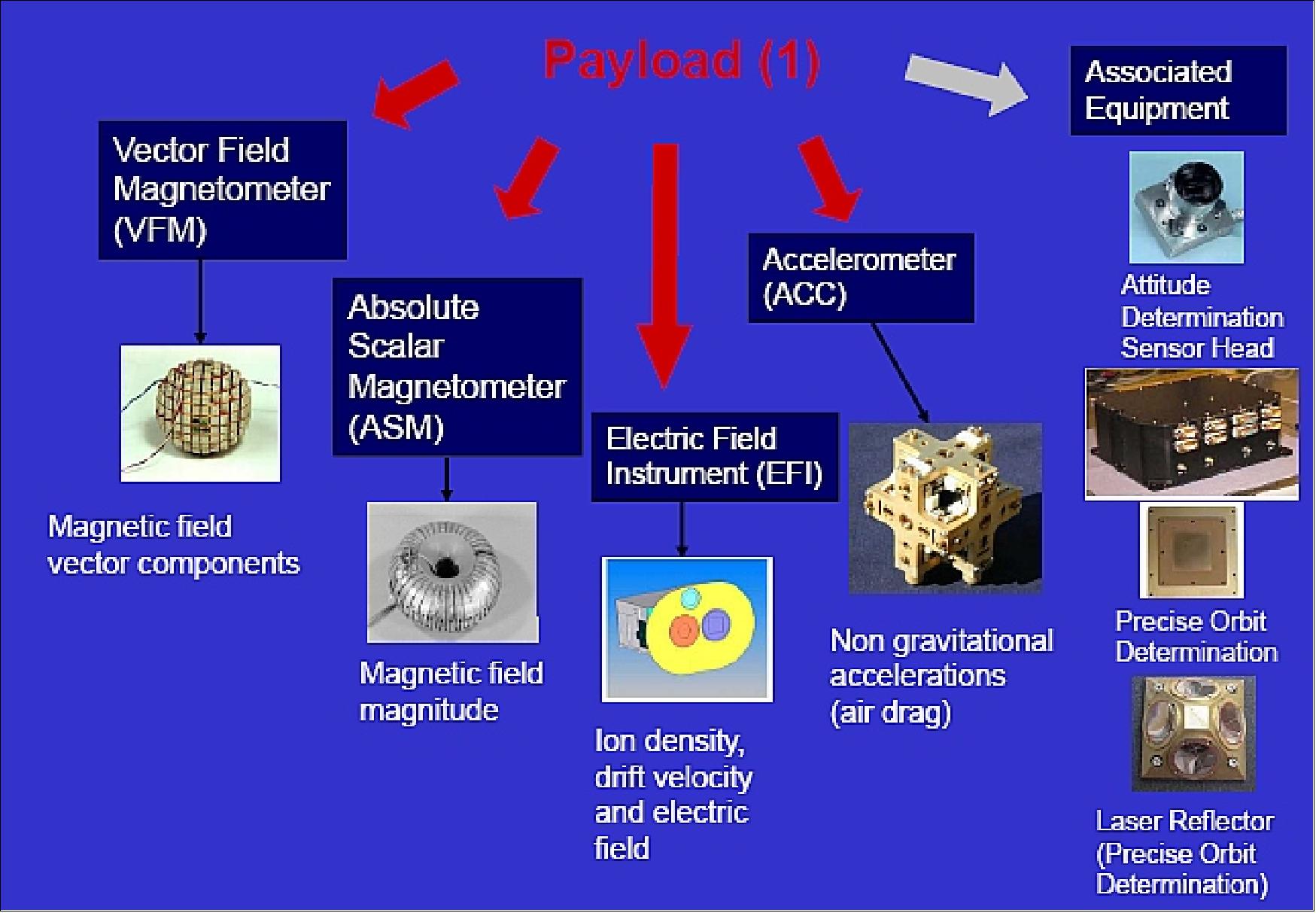
All three Swarm satellites carry the same instruments: a Vector Field Magnetometer (VFM) that measures the direction of the magnetic field; an Absolute Scalar Magnetometer (ASM) that measures the strength of the magnetic field; an Electric Field Instrument (EFI) that measures the plasma density, drift, and acceleration; as well as a Micro Accelerometer-04 (MAC-04) that measures the air drag, winds, Earth albedo, and solar radiation pressure.
Performance Specifications
VFM has a sampling rate of 50 Hz, and ASM has an absolute accuracy of less than 0.3 nT.
The first and third satellites, Swarm-A and Swarm-C, share the same non-sun-synchronous orbit with an altitude of 450 km and an inclination of 87.4°. They travel in parallel with an east-west separation of 1-1.5° and an orbital time difference of fewer than 10 seconds. The second satellite, Swarm-B, maintains a non-sun-synchronous orbit with an altitude of 530 km and an inclination of 88°.
Space & Hardware Components
Communications are performed via S-band radio frequency for Telemetry, Tracking, and Command (TT&C) as well as data transmission; the downlink data rate is 6 Mbit/s and the uplink rate is 4 kbits/s.
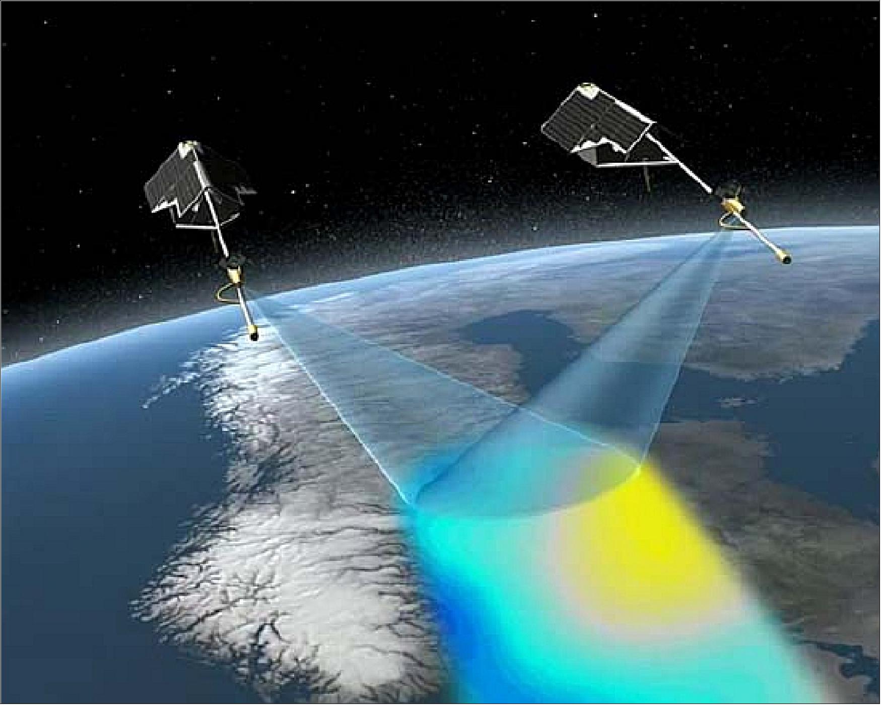
The different orbits taken by the Swarm constellation optimise the sampling in space and time to distinguish different magnetic sources and their strengths.
Swarm (Geomagnetic LEO Constellation)
Space segment concept Launch Swarm's Orbits Mission Status Sensor ComplementGround Segment References
Swarm is a minisatellite constellation mission within the Earth Explorer Opportunity Program of ESA, proposed under the lead of DNSC (Danish National Space Center) of Copenhagen, Denmark (formerly DSRI). In January 2007, DNSC became DTU Space, an institute at the Technical University of Denmark. The Swarm mission will be the 4th mission in ESA's Earth Explorer Program, following GOCE, SMOS, and CryoSat-2.
The first mission to ever map the Earth's magnetic field vector at LEO was the NASA MagSat spacecraft (launch Oct. 30 1979). Due to the low perigee (perigee=350 km, apogee=551 km), MagSat remained in orbit for only seven and a half months until June 11, 1980. About 20 years later, the Danish Ørsted micro satellite (1999-), the German CHAMP (2000-), the Argentine SAC-C (2000-) have been designed specifically for mapping the LEO magnetic field. Common to these recent missions is the magnetometry package, which utilizes a vector field magnetometer co-mounted with a star tracker (2 in the case of CHAMP) on an optical bench. As the accuracy of the instrument package has constantly increased, as well as the modelling methods have been improved towards optimized signal decomposition, it has been realized that simultaneous data from several points in space is needed, if the ultimate modelling barrier, the spatial-temporal ambiguity, has to be broken.
The overall objective of the Swarm mission is to build on the Ørsted and CHAMP mission experiences and to provide the best ever survey of the geomagnetic field (multi-point measurements) and its temporal evolution, to gain new insights into the Earth system by improving our understanding of the Earth's interior and climate. 1) 2) 3) 4) 5) 6) 7) 8) 9) 10) 11) 12) 13) 14) 15) 16) 17) 18)
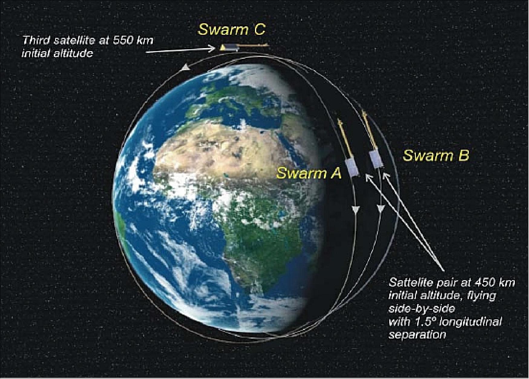
This will be done by a constellation of three satellites, two will fly at a lower altitude, measuring the East-West gradient of the magnetic field, and one satellite will fly at a higher altitude in a different local time sector. Other measurements will also be made to complement the magnetic field measurements. Together these multipoint measurements will allow the deduction of information on a series of solid-Earth processes responsible for the creation of the fields measured.
Background on the Discovery of Electromagnetism
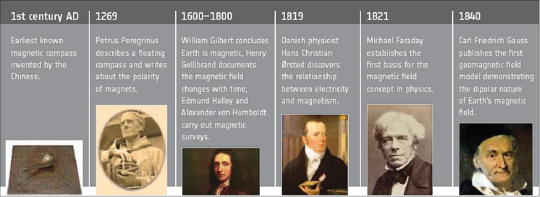
The history of magnetic discovery goes back to about 110 B.C., when the earliest magnetic compass was invented by the Chinese. They noticed that if a “lodestone” (natural magnets of iron-rich ore) was suspended so it could turn freely, it would always point in the same direction, toward the magnetic poles. This directional pointing property of magnetic material was eventually introduced into the making of an early compass and used for maritime navigation . By the 13th century, the directive property of magnetism was widely recognized and used in navigation. The mariner’s magnetic compass is the first technological application of magnetism and, one of the oldest scientific instruments.
Until 1820, the only magnetism known was that of iron magnets and of lodestones. It was the Danish physicist Hans Christian Ørsted, professor at the University of Copenhagen, who, in 1820, was first to discover the relationship between the hitherto separate fields of electricity and magnetism. Ørsted showed that a compass needle was deflected when an electric current passed through a wire, before Faraday had formulated the physical law that carries his name: the magnetic field produced is proportional to the intensity of the current. Magnetostatics is the study of static magnetic fields, i.e. fields which do not vary with time. 19) 20)
Magnetic and electric fields together form the two components of electromagnetism. Electromagnetic waves can move freely through space, and also through most materials at pretty much every frequency band (radio waves, microwaves, infrared, visible light, ultraviolet light, X-rays and gamma rays). Electromagnetic fields therefore combine electric and magnetic force fields that may be natural (the Earth's magnetic field) or man-made (low frequencies such as electric power transmission lines and cables, or higher frequencies such as radio waves (including cell phones) or television (Ref. 21).
Background on the Earth's Magnetic Field
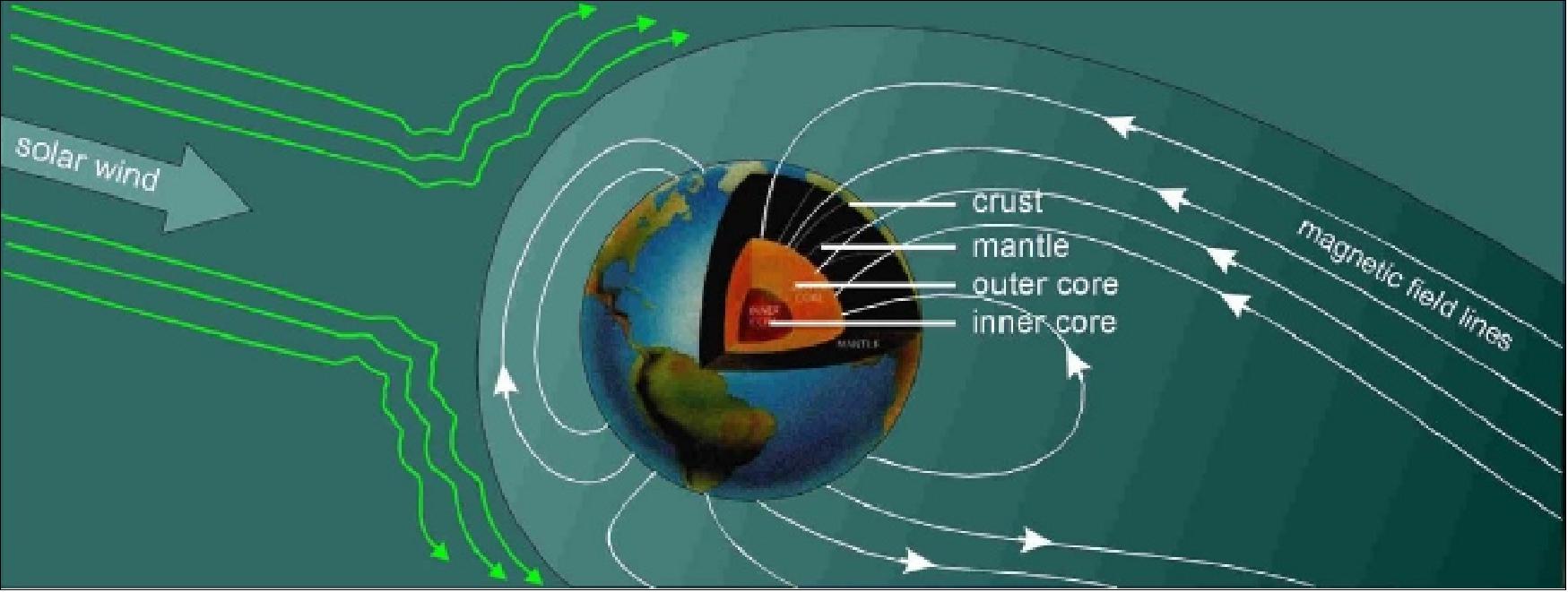
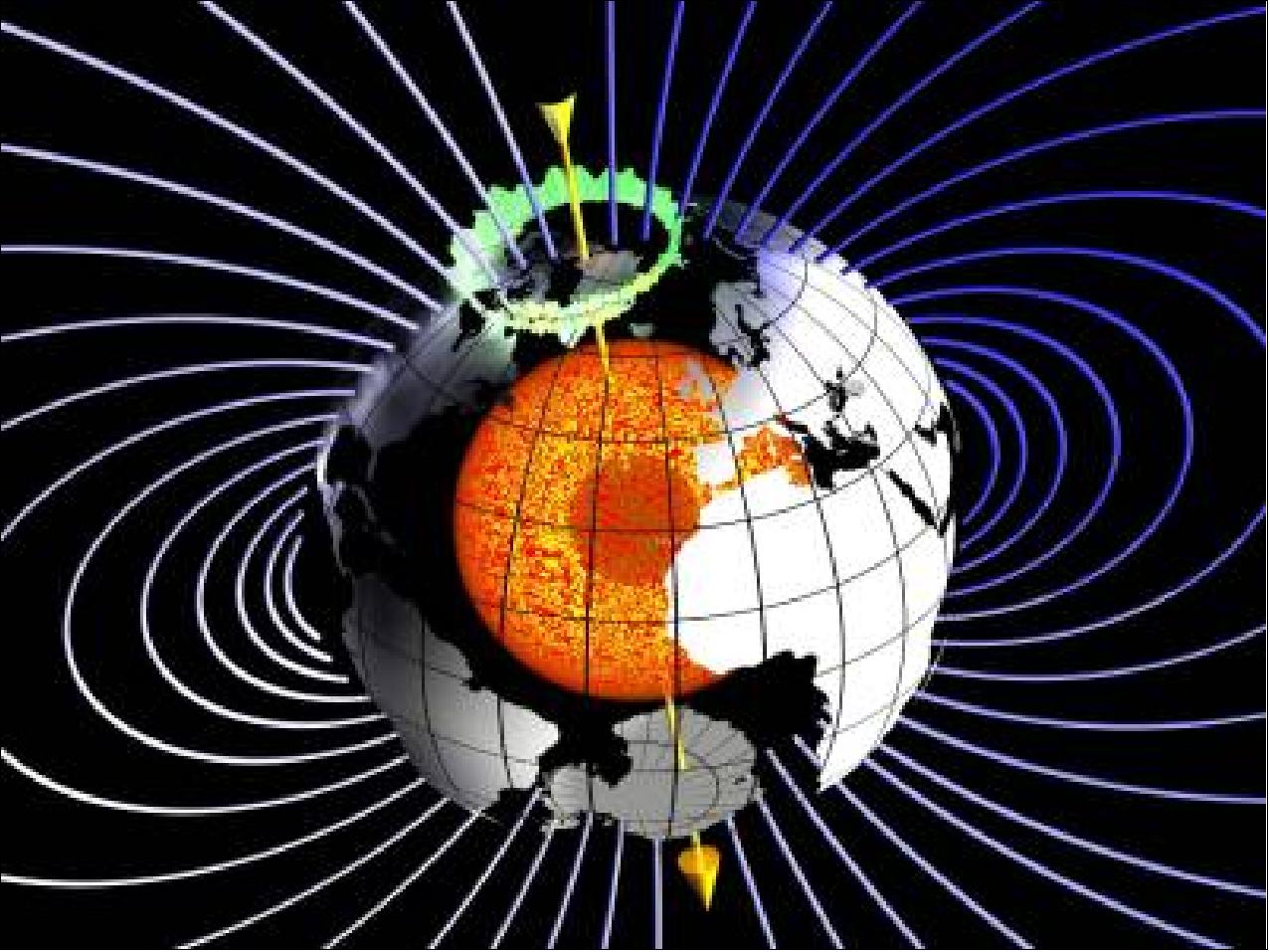
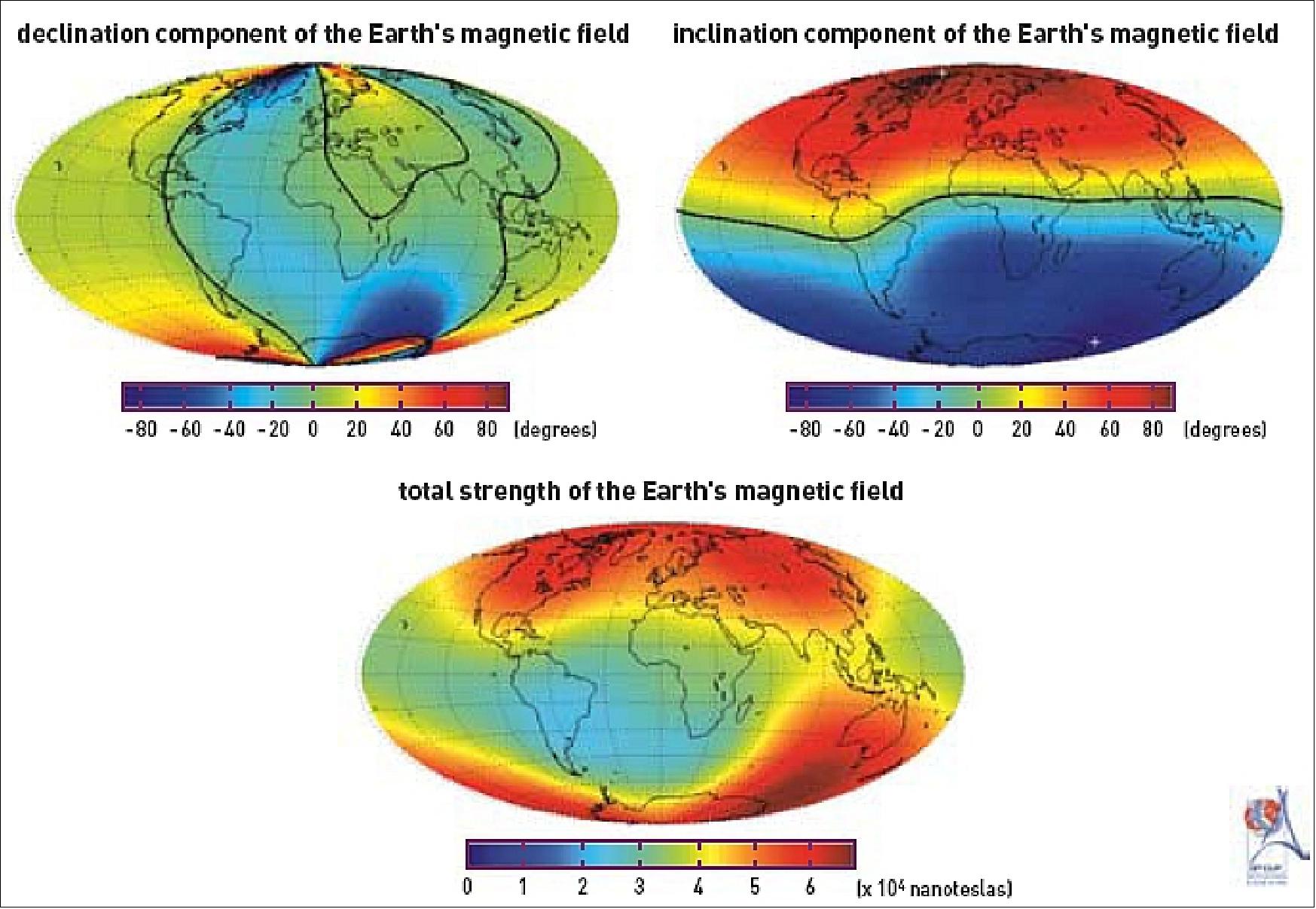
The Earth has its own magnetic field, which acts like a giant magnet. Geomagnetism is the name given to the study of this field, which can be roughly described as a centered dipole whose axis is offset from the Earth's axis of rotation by an angle of about 11.5º. This angle varies over time in response to movements in the Earth's core. The angle between the direction of the magnetic and geographic north poles, called the magnetic declination, varies at different points on the Earth's surface. The angle that the magnetic field vector makes with the horizontal plane at any point on the Earth's surface is called the magnetic inclination.
This centered dipole exhibits magnetic field lines that run between the north and south poles. These field lines convergent and lie vertical to the Earth's surface at two points known as the magnetic poles, which are currently located in Canada and Adélie Land. Compass needles align themselves with the magnetic north pole (which corresponds to the south pole of the 'magnet' at the Earth's core).
The Earth's magnetic field is a result of the dynamo effect generated by movements in the planet's core, and is fairly weak at around 0.5 gauss, i.e. 5 x 10⁻⁵ tesla (this is the value in Paris, for example). The magnetic north pole actually 'wanders' over the surface of the Earth, changing its location by up to tens of km every year. Despite its weakness, the Earth's dipolar field nevertheless screen the Earth from charged particles and protect all life on the planet from the harmful effects of cosmic radiation. In common with other planets in our solar system, the Earth is surrounded by a magnetosphere that shields its surface from solar wind, although this solar wind does manage to distort the Earth's magnetic field lines.
The Earth’s magnetic field shows deviations, called anomalies, from the idealized field of a centered bar magnet. These anomalies can be quite large, affecting areas on a regional scale. One example is the SAA (South Atlantic Anomaly), which affects the amount of cosmic radiation reaching the passengers and crew of any plane and spacecraft led to cross it (Ref. 21).
The primary research topics to be addressed by the Swarm mission include: 23)
• Core dynamics, geodynamo processes, and coremantle interaction. - The goal is to improve the models of the core field dynamics by ensuring long-term space observations with an even better spatial and temporal resolution. Combining existing Ørsted, CHAMP and future Swarm observations will also more generally allow the investigation of all magnetohydrodynamic phenomena potentially affecting the core on sub-annual to decadal scales, down to wavelengths of about 2000 km. Of particular interest are those phenomena responsible for field changes that cannot be accounted for by core surface flow models. 24)
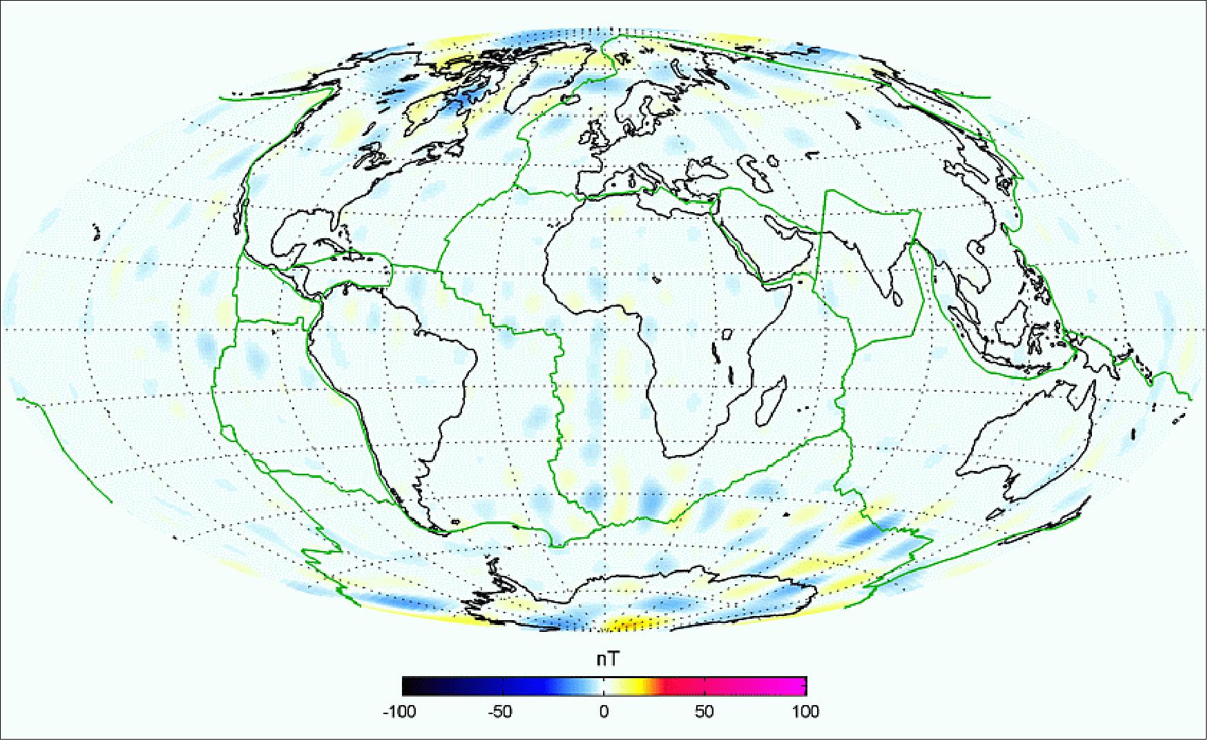
• Lithospheric magnetization and its geological interpretation. - The increased resolution of the Swarm satellite constellation will allow, for the first time, the identification from satellite altitude of the oceanic magnetic stripes corresponding to periods of reversing magnetic polarity. Such a global mapping is important because the sparse data coverage in the southern oceans has been a severe limitation regarding our understanding of plate tectonics in the oceanic lithosphere. Another important implication of improved resolution of the lithospheric magnetic field is the possibility to derive global maps of heat flux. 25) 26)
• 3-D electrical conductivity of the mantle. - Our knowledge of the physical and chemical properties of the mantle can be significantly improved if we know its electrical conductivity. Due to the sparse and inhomogeneous distribution of geomagnetic observatories, with only few in oceanic regions, a true global picture of mantle conductivity can only be obtained from space.
• Currents flowing in the magnetosphere and ionosphere. - Simultaneous measurements at different altitudes and local times, as foreseen with the Swarm mission, will allow better separation of internal and external sources, thereby improving geomagnetic field models. In addition to the benefit of internal field research, a better description of the external magnetic field contributions is of direct interest to the science community, in particular for space weather research and applications. The local time distribution of simultaneous data will foster the development of new methods of co-estimating the internal and external contributions.
The Secondary Research Objectives Include...
• Identification of the ocean circulation by its magnetic signature. - Moving sea-water produces a magnetic field, the signature of which contributes to the magnetic field at satellite altitude. Based on state-of-the-art ocean circulation and conductivity models it has been demonstrated that the expected field amplitudes are well within the resolution of the Swarm satellites. 27)
• Quantification of the magnetic forcing of the upper atmosphere. - The geomagnetic field exerts a direct control on the dynamics of the ionized and neutral particles in the upper atmosphere, which may even have some influence on the lower atmosphere. With the dedicated set of instruments, each of the Swarm satellites will be able to acquire high-resolution and simultaneous in-situ measurements of the interacting fields and particles, which are the key to understanding the system.
Historic background of Swarm: Ref. 13)
• The first Swarm proposal was made in 1998, prior to launch of the Ørsted mission.
• In early 2002, the Swarm mission was proposed to ESA by Eigil Friis-Christensen of DNSC (Copenhagen, Denmark), Hermann Lühr of GFZ (GeoForschungszentrum, Potsdam, Germany), and Gauthier Hulot of IPG (Institut de Physique du Globe, Paris, France) with support from scientists in seven European countries and the USA. In the meantime, the Swarm team comprises participation of 27 institutes on a global scale. The mission was selected for feasibility studies in 2002. The initial mission proposal considered a Swarm constellation of 4 spacecraft. 28)
• In May 2002 there were three mission candidates: ACE+, EGPM and Swarm; they were chosen for a feasibility study.
• At the end of two parallel feasibility studies, the Swarm mission was selected as the 5th mission in ESA's Earth Explorer Program in May 2004. Phase A was completed in Nov. 2005, resulting in a constellation of 3 spacecraft.
• New Concept – Constellation to characterize external sources:
- The external contributions are highly influenced by solar activity and local time
- Simultaneous satellites in different orbital planes are necessary in order to overcome the time-space ambiguity in the measurements. The optimum constellation depends on the scientific objectives.
- But, measurements of high accuracy are not sufficient! A better understanding of the various sources is equally important, in particular when doing measurements with unprecedented precision, where new phenomena appear in the data. For this, additional and independent key information is needed: a) electric field, b) ionospheric conductivity.
• In 2006, the Swarm project was in Phase B, ending with the PDR (Preliminary Design Review) in the summer 2007.
The construction of the Swarm constellation commenced in November 2007 with the Phase C/D kick-off meeting. The Swarm project CDR (Critical Design Review) took place on Oct. 14, 2008 at ESA/ESTEC. 29)
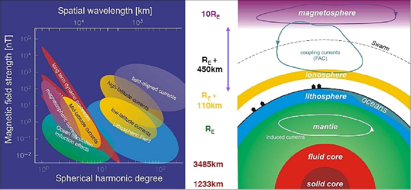
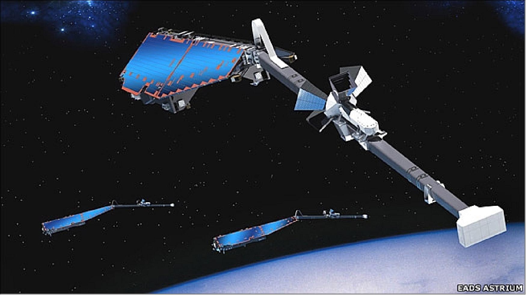
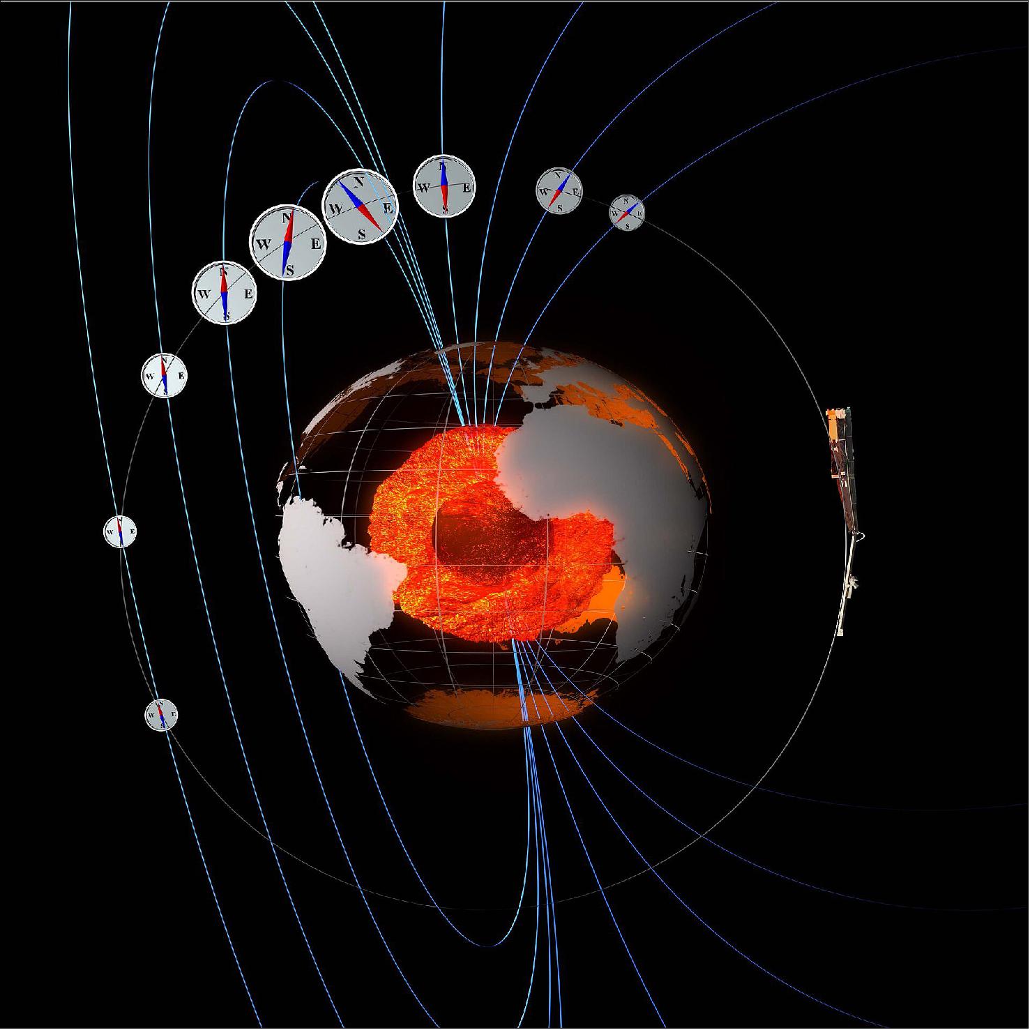
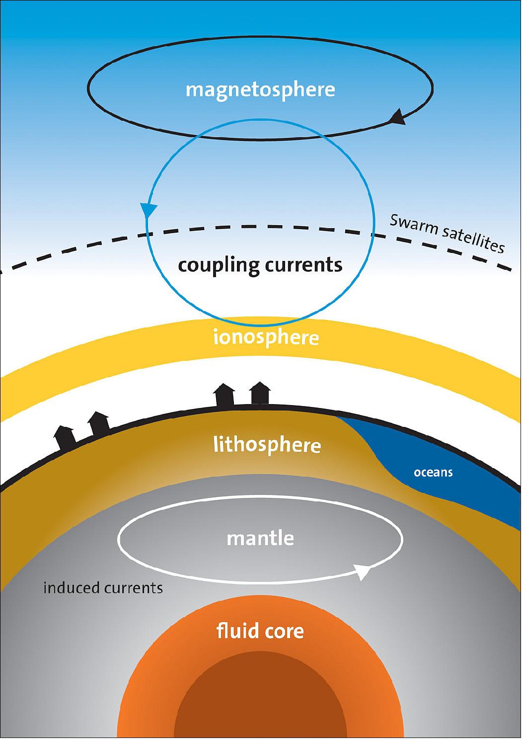
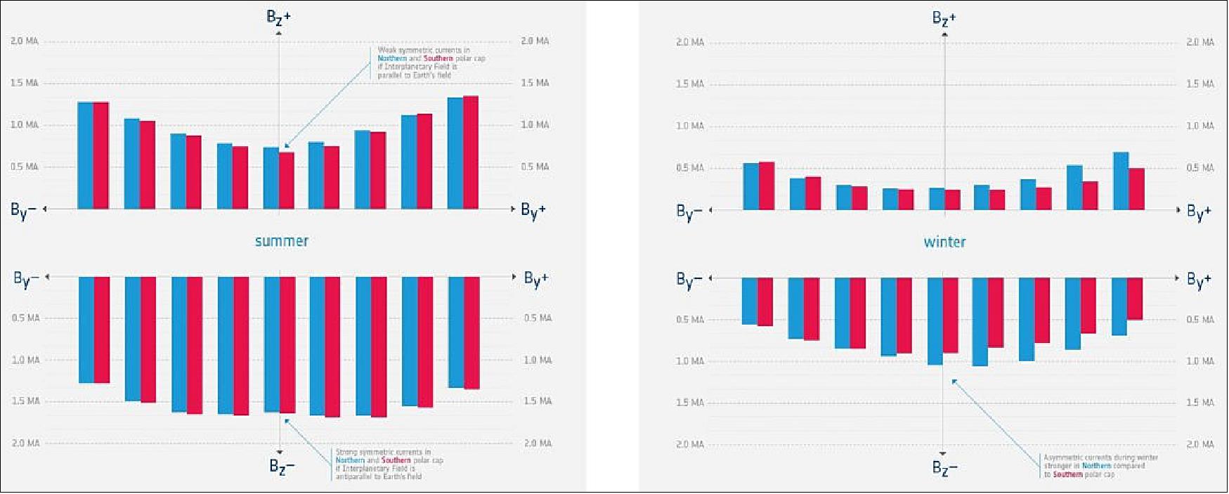
Legend to Figure 6: The magnetic field and electric currents near Earth generate complex forces that have immeasurable impact on our everyday lives. Although we know that the magnetic field originates from several sources, exactly how it is generated and why it changes is not yet fully understood. ESA’s Swarm mission will help untangle the complexities of the field.
Space Segment Concept
The Swarm mission architecture is driven by the requirement for separation of the various sources contributing to the Earth's magnetic field. Hence, the space segment concept employs a three-minisatellite constellation with the following characteristics:
- Three spacecraft in two different orbital planes, with two satellites in a plane of 84.7º inclination and with one satellite in a plane of 88º inclination
- The two satellites in the 87.4º inclination orbit will fly at a mean altitude of 450 km, their east-west separation will be 1-1.5º, and the maximum differential delay in orbit will be about 10 s.
- The satellite in the higher inclination orbit (88º) will fly at a mean altitude of 530 km.
- The spacecraft require some degree of active orbit maintenance to control the relative positions in the constellation (this is an element of formation flight to support flight operations). 31) 32)
In November 2005, ESA selected EADS Astrium GmbH, Friedrichshafen, Germany as the prime contractor for the Swarm spacecrafts. The Swarm consortium (main subcontractors) consists of: 33)
- EADS Astrium Ltd., UK (mechanical, thermal, AIV)
- GFZ Potsdam, Germany (end-to-end system simulator, calibration & validation)
- DTU Space, Copenhagen, Denmark [level 1b processor and instruments (VFM magnetometer and STR star tracker)]
The spacecraft design is governed by the following requirements:
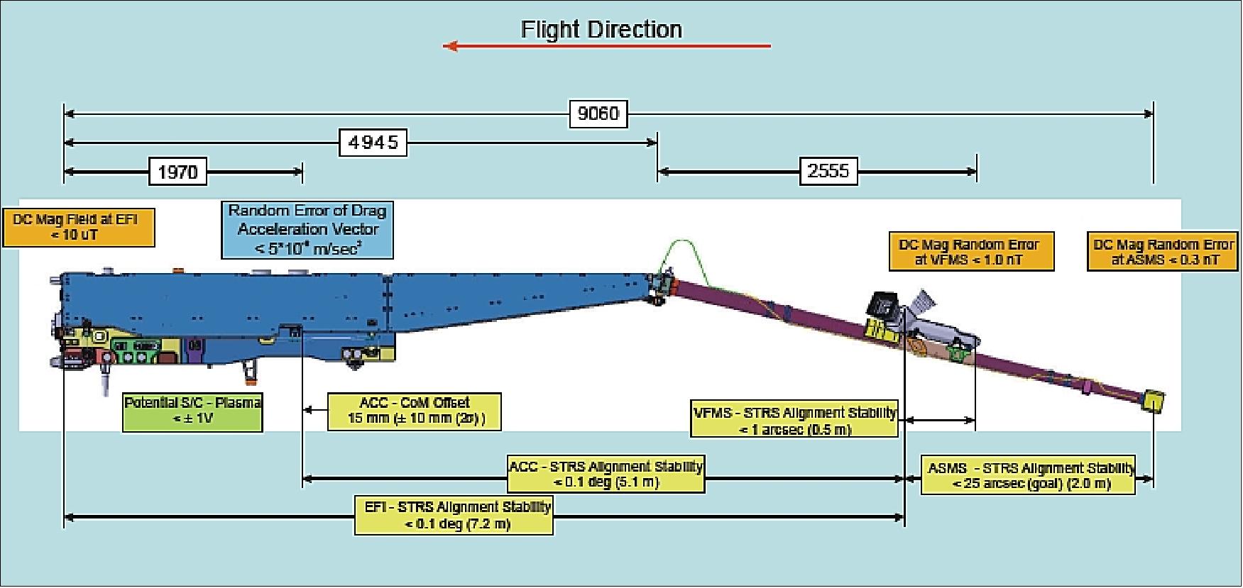
1) Magnetic cleanliness: magnetometers on deployable boom, non-magnetic materials and caution during handling
2) Magnetic field vector attitude knowledge: ultra-stable connection between VFM (Vector Field Magnetometer) and STR (Star Tracker) assembly on the optical bench
3) Ballistic coefficient: small ram surface in flight direction to minimize air drag
4) Accelerometer proof-mass vs satellite CoG (Center of Gravity) location.
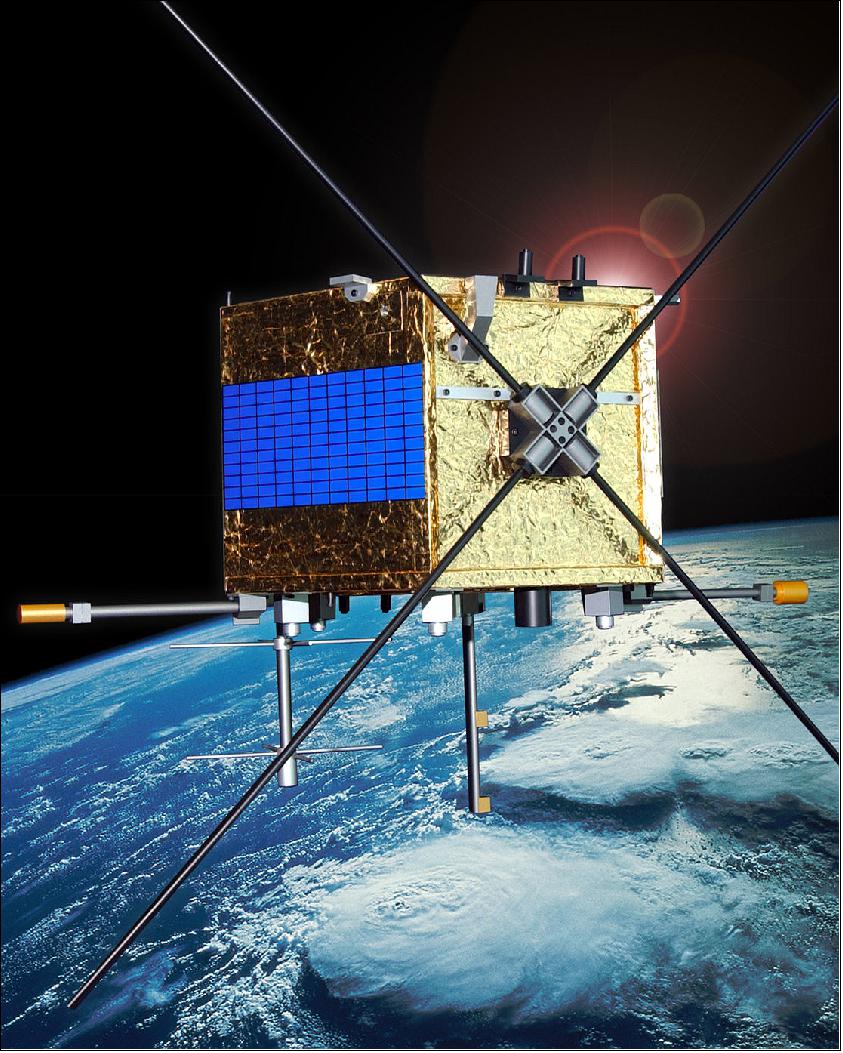
An important design measure is the accommodation of the magnetometer package at a distance from the main body/platform sufficient to minimize any magnetic disturbance. A boom ensures a magnetically 'clean' environment and provides very stable accommodation for the magnetometer package. Due to envelope constraints of the launcher fairing, the boom must be deployable. 34)
Optical bench: The vector magnetometer is mounted on an ultra-stable silicon carbide-carbon fiber compound structure (the SWARM optical bench). Both optical bench and scalar magnetometer are installed on a deployable conical tube of square cross section. The position tolerance of the optical bench to its tube interface has to be fixed within 0.2 mm. 35) 36)
The design driver of the composite tube assembly of Swarm is thermal stability. The main cause for observed thermal distortion is the non-uniformity of the cross-sections arising from the different adaptations of the filament winding process in order to manufacture the carbon fiber reinforced structure. The manufacture of the structure required use of thermally controlled high precision bonding jigs to join the composite tubes to the metallic fittings.
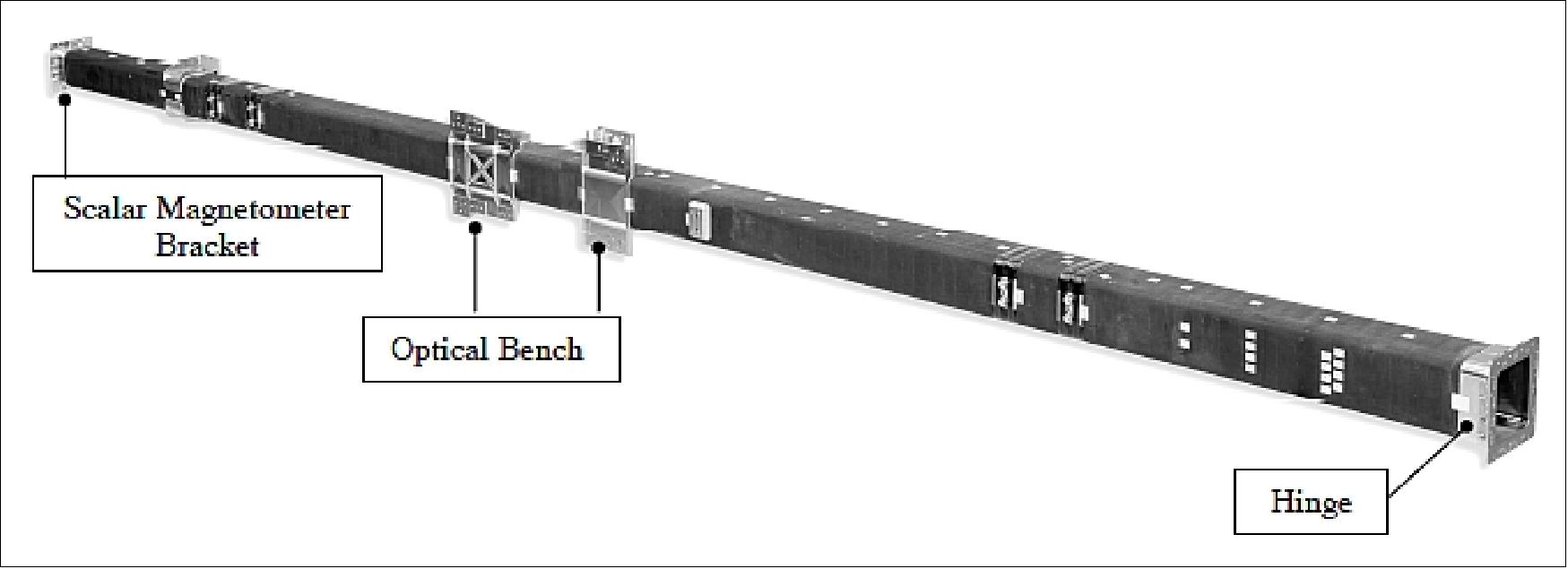
The scalar magnetometer and optical bench are fixed to a deployable large beam of square cross section, the SWARM (Carbon-fiber Tube Assembly (CTA) which fulfils the following main functions (Figure 8):
• Separate the sensitive instruments from the spacecraft to comply with the very high magnetic cleanliness requirements
• Provide a suitable stable structure for the fixation of instruments.
The chosen manufacturing technology for the SWARM tube was filament winding. The SWARM tube has a conical taper. Since the amount of fibers in a cross section is constant the tube had two main characteristics: the wall thickness increased linearly from the root to the tip and due to nature of the winding process the fiber angle became steeper at the tip than at the root. The overall effect is a variation of properties along the length of the tube.
The Swarm carbon-fiber tube assembly was subjected to various tests: Thermal distortion was measured by establishing a 65ºC gradient between the tip and the hinge and a 10ºC gradient between opposite sides of the CTA. The hole pattern of the optical bench was accurate to within 0.2 mm (Ref. 35).
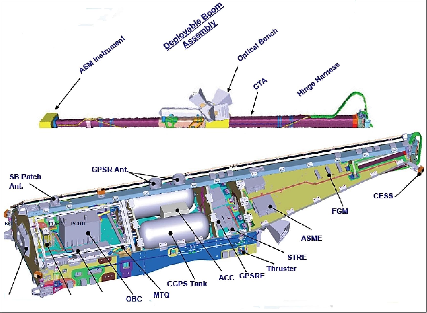
The three identical Swarm minisatellites consist of the payload and the platform elements. The platform comprises the following subsystems: structure/mechanisms, power, RF communications, AOCS (Attitude and Orbit Control Subsystem), thermal control, and onboard data handling.
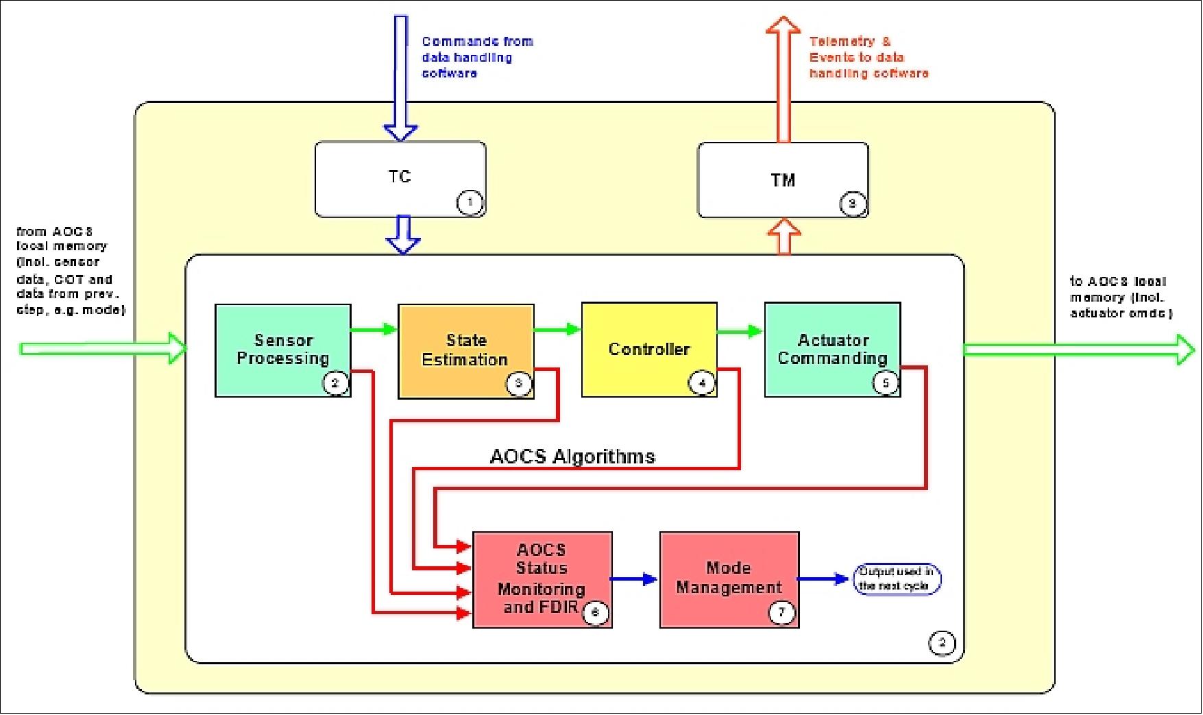
The AOCS design is based to a maximum extent on the CryoSat AOCS design of EADS Astrium. The gyro-less AOCS provides 3-axis stabilization with an Earth pointing attitude control in all modes. The requirements call for: 37)
- An attitude pointing control within a band of < 5º about all axis (roll, pitch, and yaw), the pointing stability is < 0.1º/s
- Provision of a sufficient torque capability for launcher tip-off rate damping and attitude acquisition
- Minimize acceleration and magnetic stray field disturbances to scientific instruments
- Provision of a high ΔV capability for orbit & attitude control maneuvers.
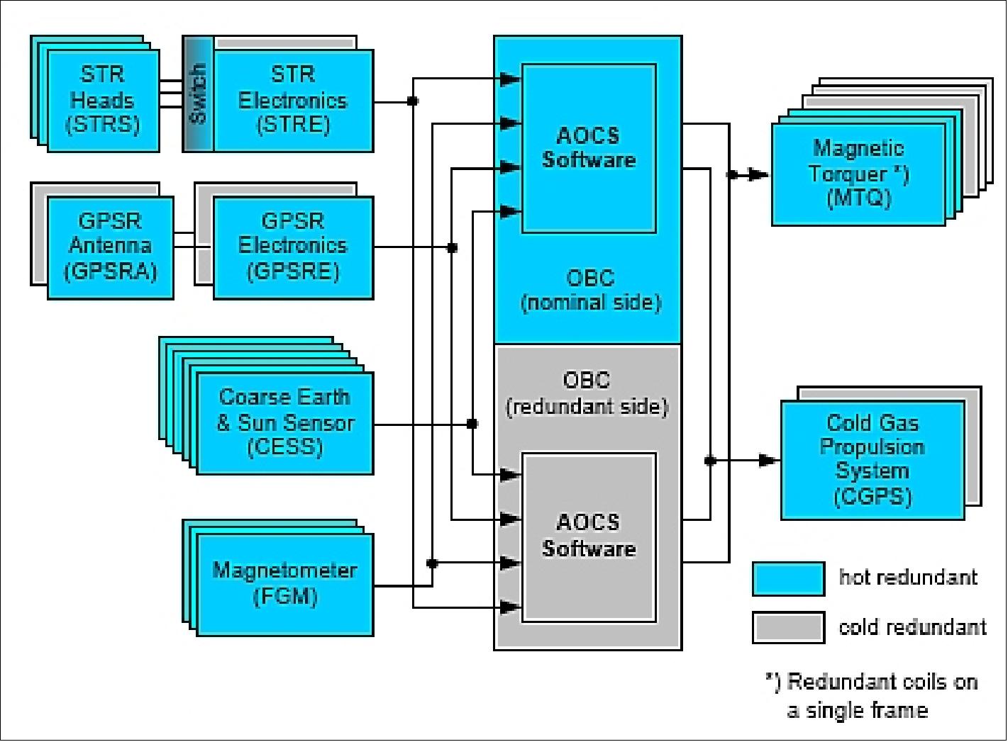
The AOCS is tightly coupled with the propulsion subsystem. Actuation is provided by a cold gas propulsion subsystem, referred to as OCS (Orbit Control Subsystem), and magnetic torquers (used for ΔV maneuvers and to complement the magnetic torquers). The cold gas propulsion system is provided by AMPAC-ISP, UK. - Attitude sensing is provided by a star tracker assembly (3 star tracker heads), 3 magnetometers, and a CESS (Coarse Earth and Sun Sensor) assembly used in safe mode situations and in initial acquisition sequences, respectively (CESS is of CHAMP, GRACE, and TerraSAR-X heritage). A dual frequency GPS receiver (GPSR) is used to provide PPS (Precise Positioning Service) to the OBC and instruments for on-board datation.
Note: the star tracker (STR) assembly and optical bench are described below under a separate heading.
The nominal attitude has a nadir orientation. Rotation maneuvers of S/C about roll, pitch and yaw are used for instrument calibration and orbit Control. The safe mode is Earth-oriented. Pointing requirements are 2º about all axes, with limitations on use of actuators.
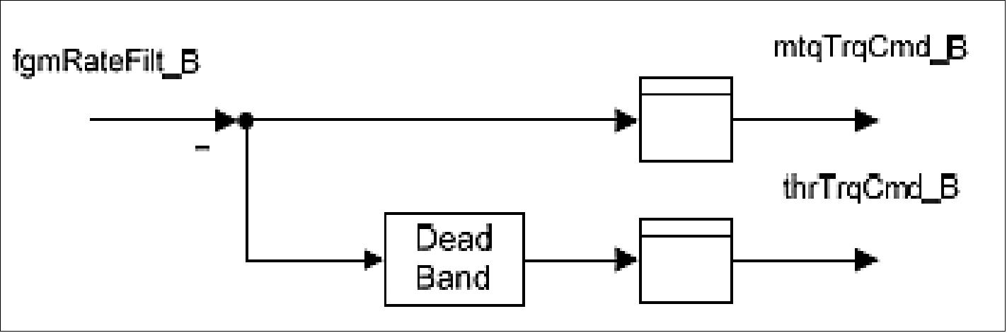
The Swarm rate damping design, in support of the critical spacecraft deployment phase, employs magnetic rate damping - magnetometers in combination with magnetic torquers and thrusters - to provide a significantly cheaper implementation than with the use of gyroscopes. From a control theory point-of-view, rate damping with magnetometers using 2-axis measurement is as “safe” as with gyroscopes using 3-axis measurement: Global asymptotical stability is achieved except for the case when the magnetic field does not change. This is only in near-equator orbits possible with perfect field symmetry which is in practice not realistic. The result is confirmed by the evaluation of the observability criterion where no loss of this property could be detected except for the mentioned case. Since SWARM is in a polar inclination orbit, the control concept is considered “clean”. 38)
Rate damping design: The RDM controller is a simple proportional controller on the S/C rate with reference rate zero. The S/C rate is computed by processing and derivation of the FGM measurements. The controller outputs the torque commands for the torquer and the thruster. A dead band for the thruster inhibits the thruster activation for low rates which can be covered by the torque rod.
Each spacecraft features 2 propellant tanks, each with a capacity of 30 kg of N2. The thrusters provide thrust levels of 20 and 40 mN. The cold gas thruster system was developed and space qualified by Ampec-ISP, Cheltenham, UK consisting of 24 OCT (Orbit Control Trusters) and 48 ACT (Attitude Control Thrusters) for the Swarm constellation. The assembly and test of Ampac's SVT01 series of cold gas thrusters has included design modifications, full qualification and verification of suitability to operate with a new propellant. In 2010, a set of 72 units has been supplied and integrated into the constellation of three Swarm spacecraft. 39)
A GPS receiver provides the functions of timing and position determination. The spacecraft dry mass is about 370 kg.
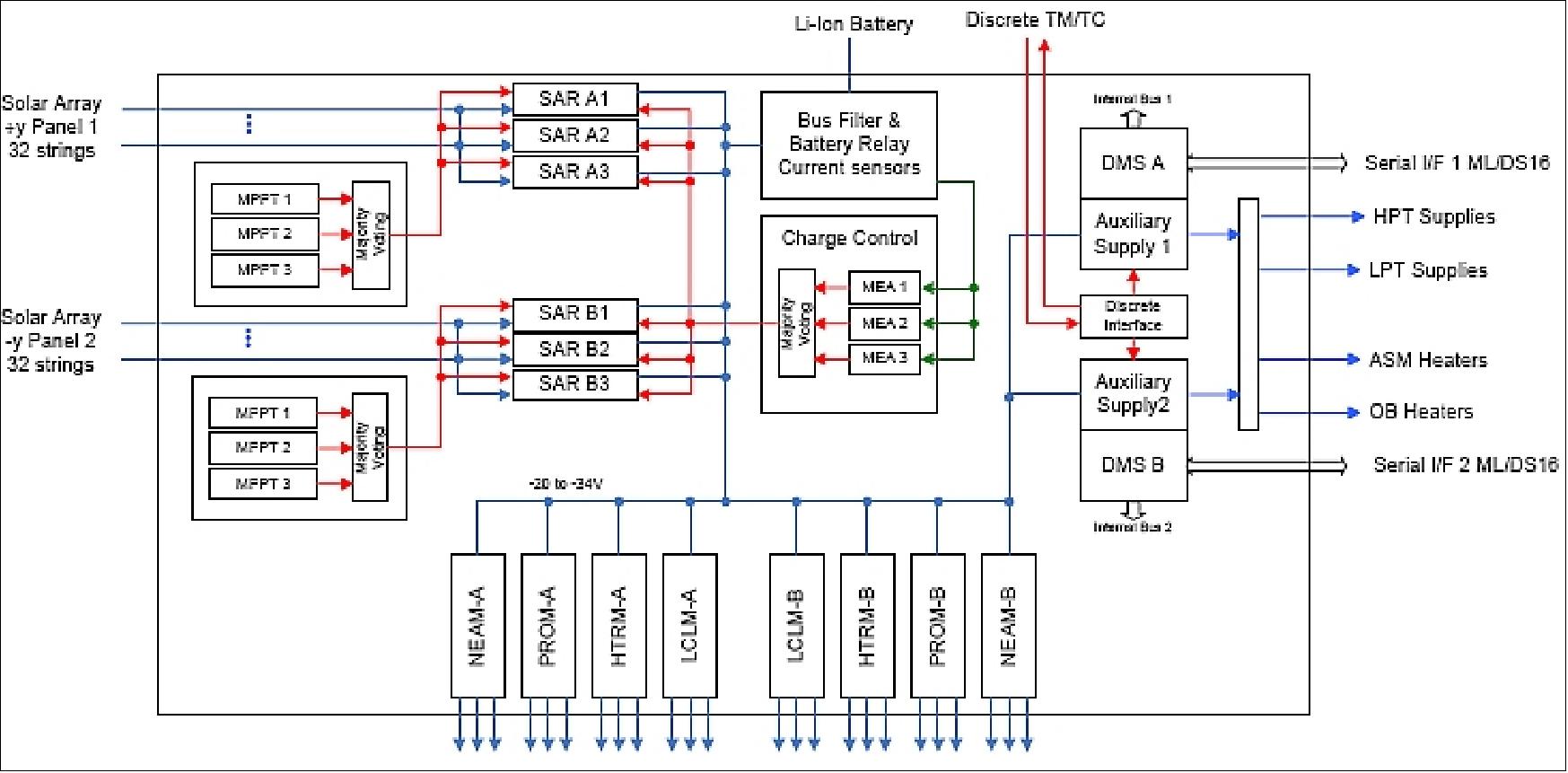
EPS (Electrical Power Subsystem): The two body-mounted solar arrays and the varying orbits of the satellites require a MPPT (Maximum Power Point Tracking) system. Important requirements are related to the magnetic cleanliness of the satellites and result in following specific PCDU (Power Conditioning and Distribution Unit) design requirements: 40)
- Minimization of magnetic moment i.e. minimizing of magnetic materials and current loops
- Selection of switching frequencies outside the ‘forbidden’ frequency ranges
- Minimizing spacecraft surface charging by use of negative bus voltage concept (battery + is connected to spacecraft structure).
The PCU part of the PCDU covers all tasks to control the power flow in the unit from the different sources and performs the communication with the OBC (On Board Computer).
During eclipse and battery recharge mode, the bus voltage varies with the state of charge of the battery. In taper charge mode, the bus is controlled by the MEA (Main Error Amplifier) to a predefined (commandable) value.
The main power requirements for the PCDU are defined as follows:
- Solar array input: 0 to -125 V, max. 21 A (each of 2 panels)
- Maximum power per panel: 750 W
- Main bus voltage range -22 V to -34 V
- Maximum battery charge current 24 A
- Continuous discharge current 0 to 14 A.
Maximum discharge current/power up to 0.5 h: 20 A / 440 W.
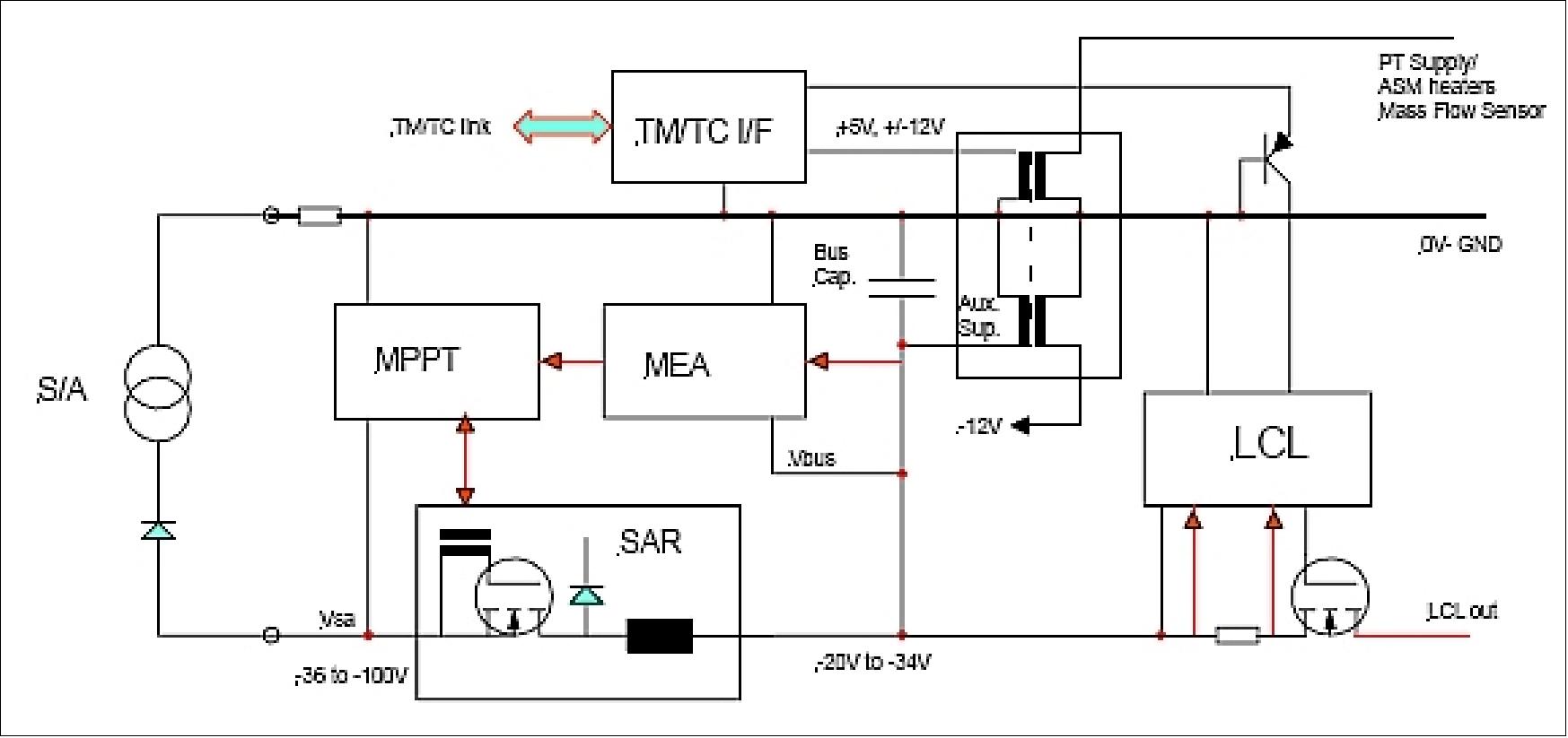
Negative bus voltage concept: The Swarm satellite requires the positive line of the power system connected to structure. This implies that all bus protection functions have to be allocated in the ‘hot’ negative line. As all essential functions, ( i.e. bus voltage control) need to be independent from the auxiliary supplies, they have to be supplied by the negative bus voltage. Figure 15 shows a principle grounding/power supply diagram of the main functional blocks in the PCDU.
Power control concept: The PCDU uses a simple concept for control of the battery state of charge and the bus voltage:
- Whenever the bus voltage and the charge current are below the limits, the MPPTs are active
- When the either the bus voltage attains the ‘battery end-of-charge voltage or the battery attains the charge current limit, the MEA (Main Error Amplifier) supersedes the tracker operation.
A bus overvoltage detection logic has been implemented in the PCDU, which performs a rapid ramp-down of the solar regulator current by using hysteresis control.
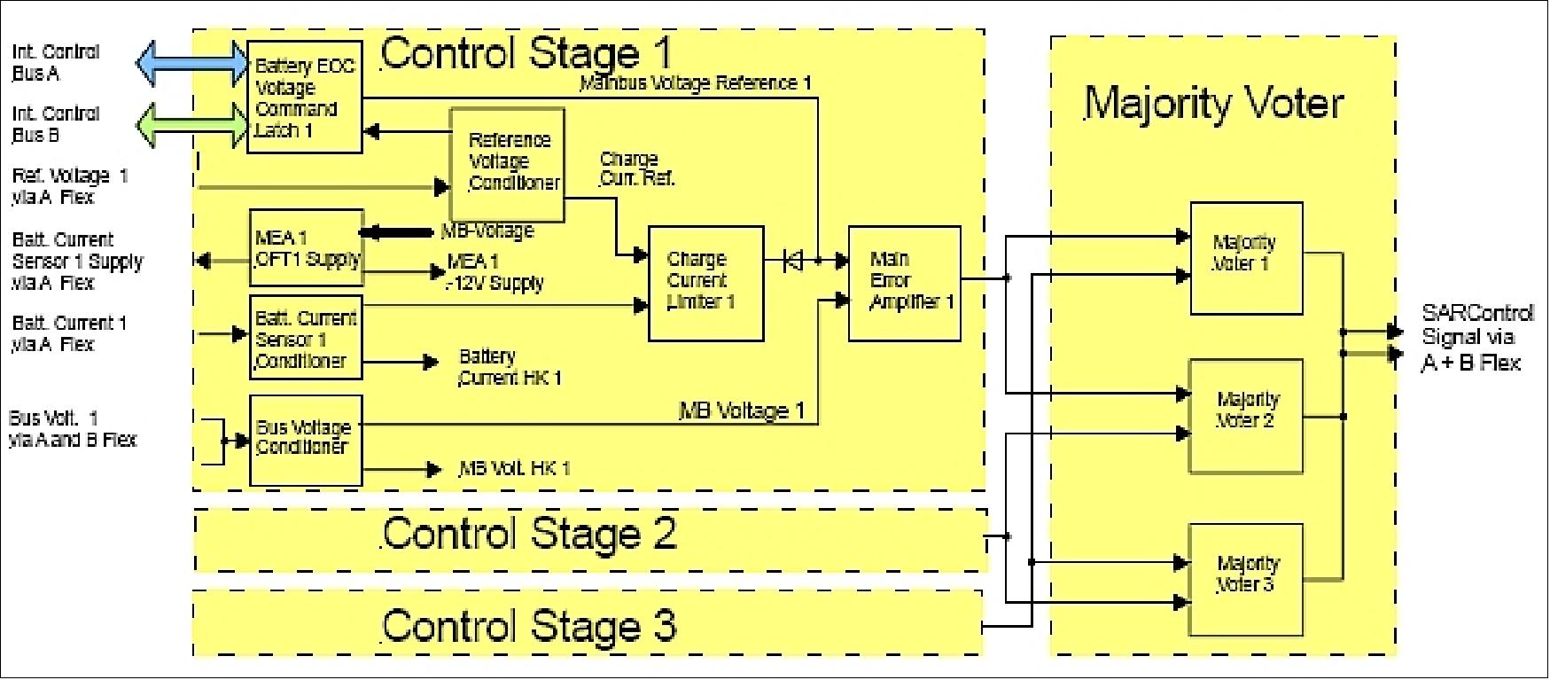
The MEA is composed of 3 identical separated control stages and a majority voter. Each control stage has a dedicated set of sensors and receives the relevant set commands for the bus voltage via redundant internal control busses. The charge current limitation is implemented in a ‘cascade configuration’, using the output of the current error amplifier as a set signal for the voltage amplifier. This assures a low and constant bus impedance during all MEA control modes. The implementation of the regulation concept is given in Figure 16.
Spacecraft mass | Dry mass of ~369 kg |
Spacecraft dimensions | Length: 9.1 m; width: 1.5 m (S/C body); height: 0.85 m; ram surface: ~0.7 m2 |
Boom length | 5.1 m |
AOCS | - 3-axis stabilized; magnetometers; CESS; GPS; STR, magnetorquers; thrusters |
AOCS sensors | - STR (Star Tracker) with 3 sensor heads |
AOCS control modes | - Rate damping: rates are measured by the FGMs, main actuation by THR |
EPS (Electrical Power Subsystem) | Total power: 608 W nominal; solar cells: GaAs triple junction; solar panel positive grounding; a set of batteries: Li-ion with a capacity of 48 Ah |
RF communications | S-band; downlink data rate: 6 Mbit/s; 4 kbit/s uplink, data volume: 1.8 Gbit/day; 1 dump/day to Kiruna ground station, data storage capability: 2 x 16 Gbit |
Mission duration | 3 months of commissioning followed by 4 years of nominal operations |
RF communications: S-band for TT&C spacecraft monitoring services and for science data transmission.
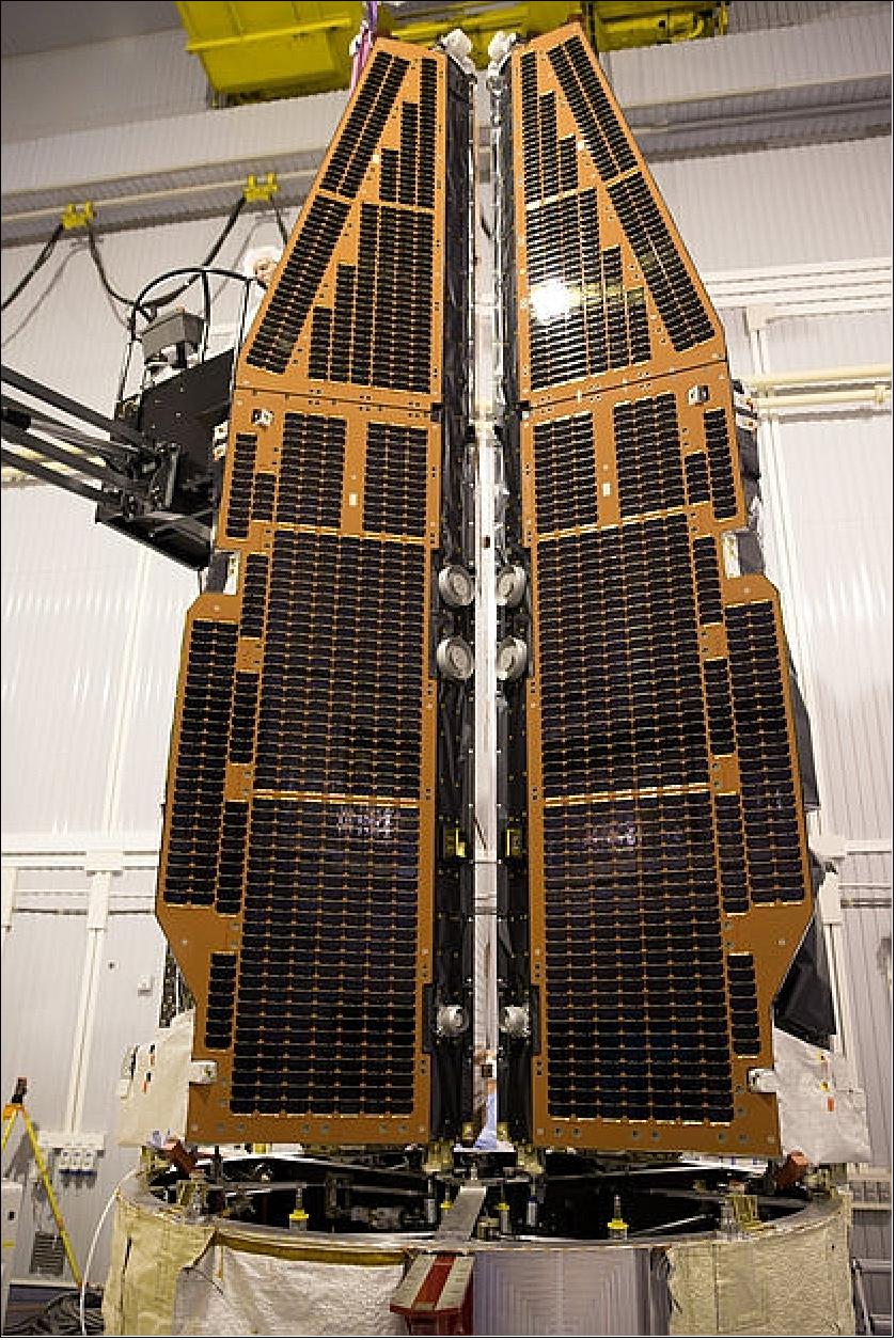
Legend to Figure 19: Attached to the tailor-made launch adapter, the three Swarm satellites sit just centimeters apart. This novel part of the rocket keeps the satellites upright within the fairing during launch and allows them to be injected simultaneously into orbit. 41)
DBA (Deployable Boom Assembly): The Swarm DBA, consisting of a 4.3m long CFRP tube and a hinge assembly, is designed to perform this function by deploying the CFRP tube plus the instruments mounted on it. mounted on a 4.3m long deployable boom. Deployment is initiated by releasing 3 HDRMs (Hold Down Release Mechanisms) , once released the boom oscillates back and forth on a pair of pivots, similar to a restaurant kitchen door hinge, for around 120 seconds before coming to rest on 3 kinematic mounts which are used to provide an accurate reference location in the deployed position. The motion of the boom is damped through a combination of friction, spring hysteresis and flexing of the 120+ cables crossing the hinge. Considerable development work and accurate numerical modelling of the hinge motion was required to predict performance across a wide temperature range and ensure that during the 1st overshoot the boom did not damage itself, the harness or the spacecraft. - Due to the magnetic cleanliness requirements of the spacecraft, no magnetic materials could be used in the design of the hardware. 42)
Launch
The Swarm constellation was launched on Nov. 22, 2013 (12:02:29 UTC) on a Rockot vehicle from the Plesetsk Cosmodrome, Russia. The launch was provided by Eurockot Launch Services. Some 91 minutes after liftoff, the Breeze-KM upper stage released the three satellites into a near-polar circular orbit at an altitude of 490 km. 43) 44) 45) 46) 47)
The launch was planned for the fall of 2012, but due to the recent Breeze-M (Briz-M) failure the launch was postponed to permit proper investigations of the cause. In Nov. 2012, ESA is still expecting, from the Russian Ministry of Defence, the launch manifest for the year 2012/13 for Rockot launchers indicating the launch date for Swarm. 48) 49)
Note: Rockot, a converted SS-19 ballistic missile, has been grounded since February 1, 2011 when the Rockot vehicle with the Breeze-KM upper stage failed to place the Russian government’s GEO-IK2 geodesy satellite of 1400 kg (Kosmos 2470) into its intended orbit of 1000 km. However, in the meantime, the Rockot/Breeze-KM vehicle demonstrated its reliability by lifting 4 Russian spacecraft (Gonets-M No.3, Gonets-M No.4, Strela-3/Rodnik, and Yubileiny-2/MiR) successfully into orbit on July 28, 2012.
On April 9, 2010, ESA awarded a contract to Eurockot, for the launch of two of its Earth observation missions. The contract covers the launch of ESA's Swarm magnetic-field mission and a 'ticket' for one other mission, yet to be decided. Both will take place from the Plesetsk Cosmodrome in northern Russia using a Rockot/Breeze-KM launcher. Eurockot is based in Bremen, Germany and is a joint venture between Astrium and the Khrunichev Space Center, Moscow. 50) 51) 52) 53)
After release from a single launcher, a side-by-side flying lower pair of satellites at an initial altitude of 460 km and a single higher satellite at 530 km will form the Swarm constellation. The constellation deployment and maintenance require a total ΔV effort of about 100 m/s.
In LEOP (Launch and Early Orbit Phase), at least three ground stations will be involved. LEOP is expected to last 3 days for the full activation of the satellites, followed by an orbit acquisition phase of up to three months. In parallel with the orbit acquisition phase, the commissioning phase will start in order to check out all satellite subsystems and the payload. The commissioning phase is currently expected to last three months. After the commissioning phase the nominal mission phase of 4 year starts.
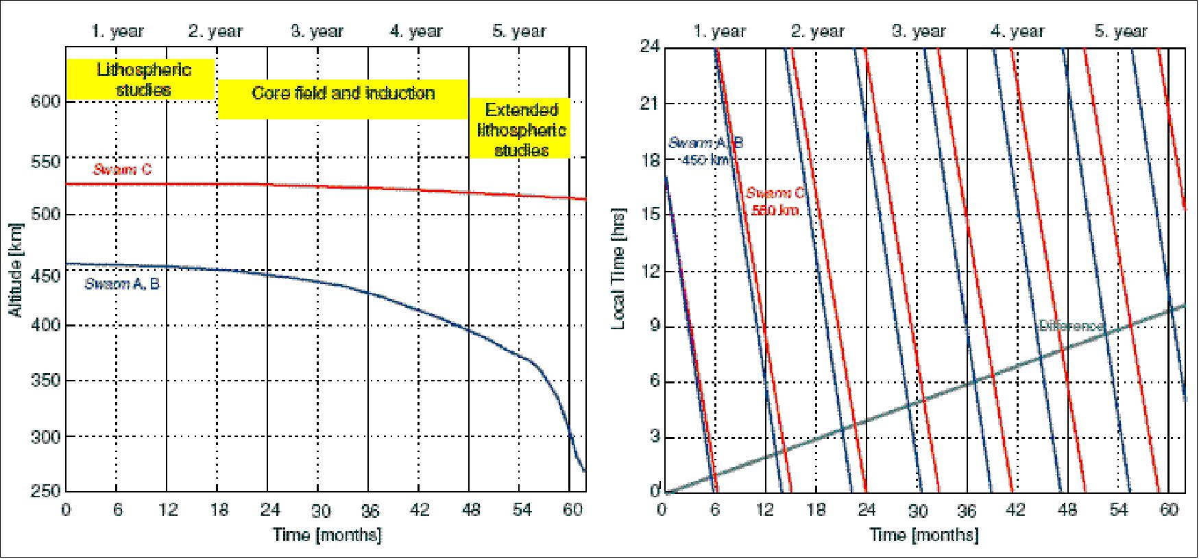
Orbits of the Swarm Constellation
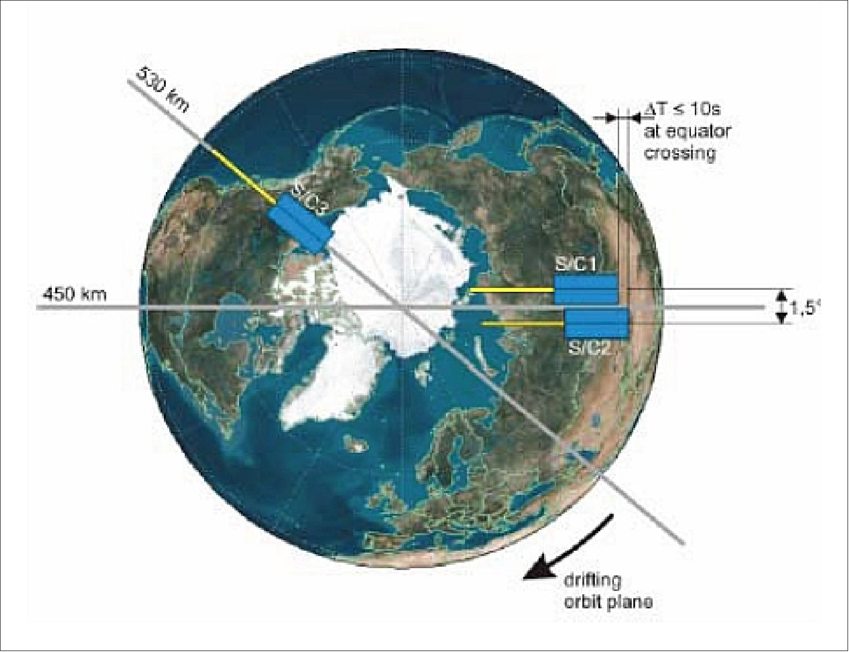
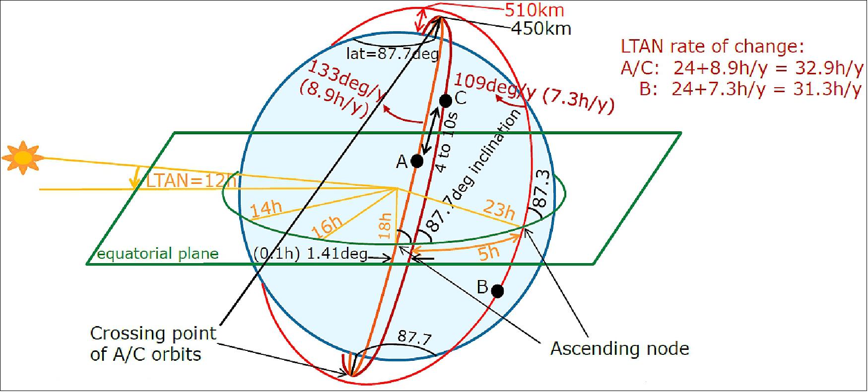
Accurate determination and separation of the large-scale magnetospheric field, which is essential for better separation of core and lithospheric fields, and for induction studies, requires that the orbital planes of the spacecraft are separated by 3 to 9 hours in local time. For improving the resolution of lithospheric magnetization mapping, the satellites should fly at low altitudes - thus experiencing some drag, but commensurate with the goals of a multi-year mission lifetime. The three satellites are being flown in 3 orbital planes with 2 different near-polar inclinations to provide a mutual orbital drift over time (Figure 20 and 21).
• Two satellites (Swarm A+B) are in a similar plane of 87.4º inclination. The satellite pair of 87.4º inclination will fly at a mean altitude of 450 km, their east-west separation shall be 1-1.4º, and the maximal differential delay in orbit shall be about 10 s. The formation-flying aspects concern the satellite pair, a side-by-side formation, requiring some formation maintenance.
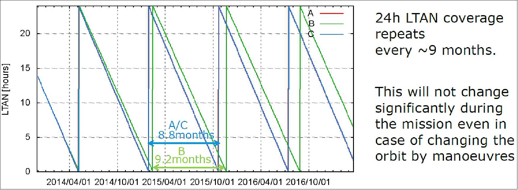
• One higher orbit satellite (Swarm C) in a circular orbit with 88º inclination at an initial altitude of 530 km. The right ascension of the ascending node is drifting somewhat slower than the two other satellites, thus building up a difference of 9 hours in local time after 4 years.
Note: Due to ASM instrument problems on Swarm-C (Charlie), it was decided prior to launch to place Charlie with Alpha on the lower orbit, and Bravo on the higher orbit.
Parameter | Swarm-A (Alpha) | Swarm-C (Charlie) | Swarm-B (Bravo) |
Orbital altitude | ≤ 460 km (initial altitude of satellite pair) | ≤ 530 km | |
Orbital inclination | 87.4º | 88º | |
ΔRAAN (Right Ascension of Ascending Node) | 1.4º difference between A and B | ~0-135º difference | |
Mean anomaly at epoch | Δt = 2-10 s difference between A and B | N/A | |
LTAN evolution (Figure 20, right-hand side) | 24 hours of local time coverage every 7-10 months | ||
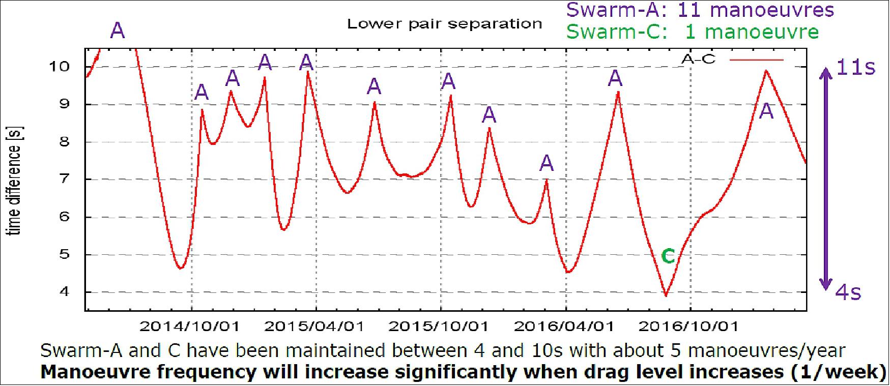
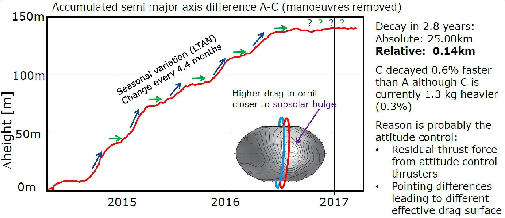
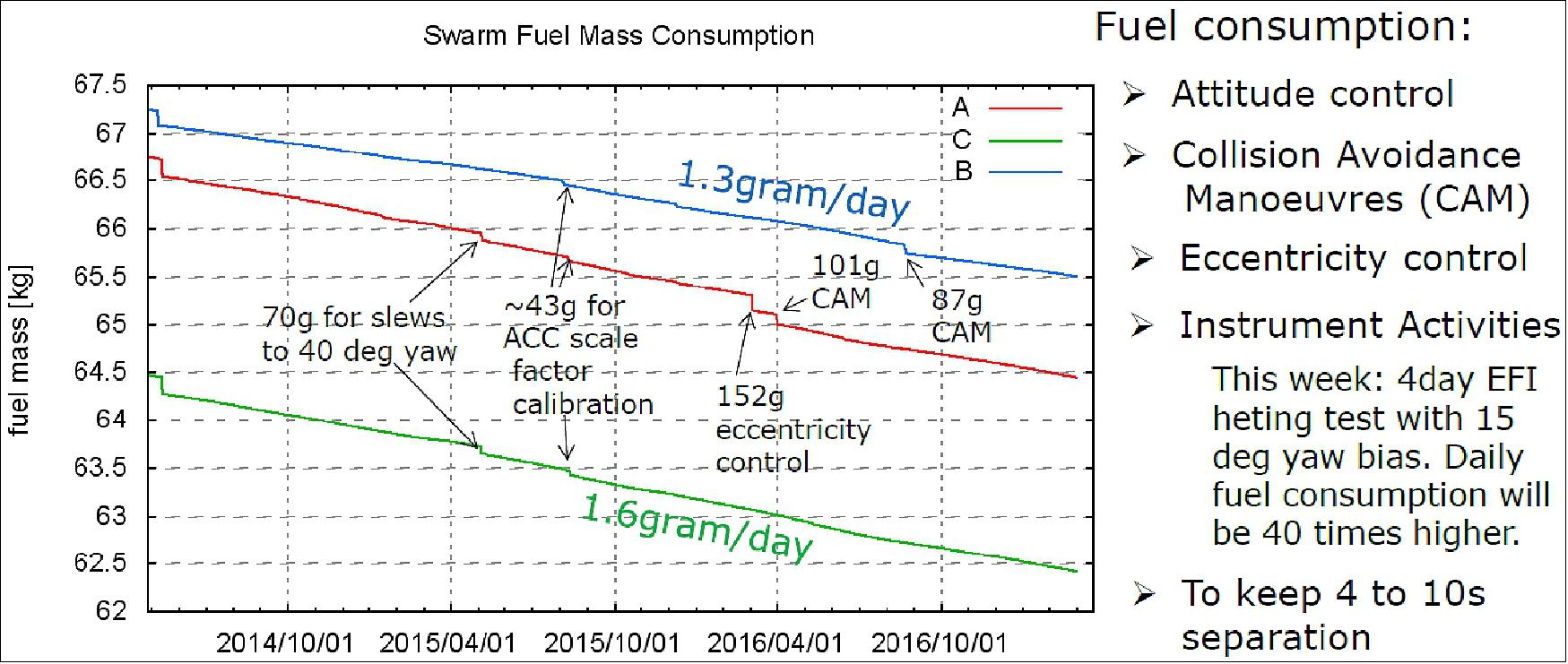
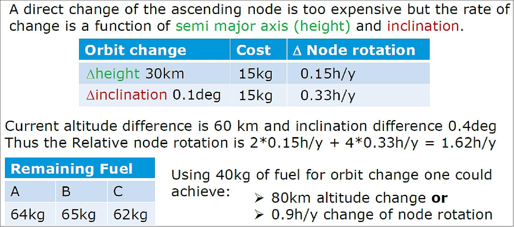
Swarm Mission Orbit Update Information as of March 2017
The following 8 Figures (Figure 24 to 32), dealing with the Swarm constellation flight dynamics, were provided by Detlef Sieg of ESA. They were presented at the 4th Swarm Science Meeting & Geodetic Workshop in Banff, Canada. 56)
Mission Status
• March 26, 2024: ESA's space weather monitoring efforts received a significant boost as the unlikely duo of SMOS and Swarm collaborated to track a severe solar storm that affected Earth's magnetic field. The solar event, initiated by a powerful X1.1 solar flare, prompted swift action from scientists and provided valuable insights into the dynamics of space weather. SMOS, originally designed for Earth observation, showcased its versatility by detecting solar radio bursts associated with the flare, while Swarm's magnetometers captured changes in Earth's magnetic field. This collaborative effort underscores the importance of ESA's Earth Explorer missions in advancing our understanding of space weather phenomena and their impact on our planet, with future initiatives like the Vigil mission poised to enhance early warning capabilities. 163)
• July 14, 2022: ESA's Swarm mission faced a close call as one of its satellites, Alpha, narrowly avoided a collision with space debris detected just eight hours before potential impact. This event highlights the ongoing challenge of space debris threatening satellites in orbit. Despite limited notice, the Swarm team swiftly orchestrated an evasive manoeuvre, ensuring Alpha's safety and preserving the mission's scientific objectives. This incident underscores the importance of proactive measures to mitigate the growing issue of space debris, including enhanced tracking technology, computational tools for manoeuvre planning, and efforts to prevent further debris accumulation through sustainable practices and potential debris removal strategies. 57)
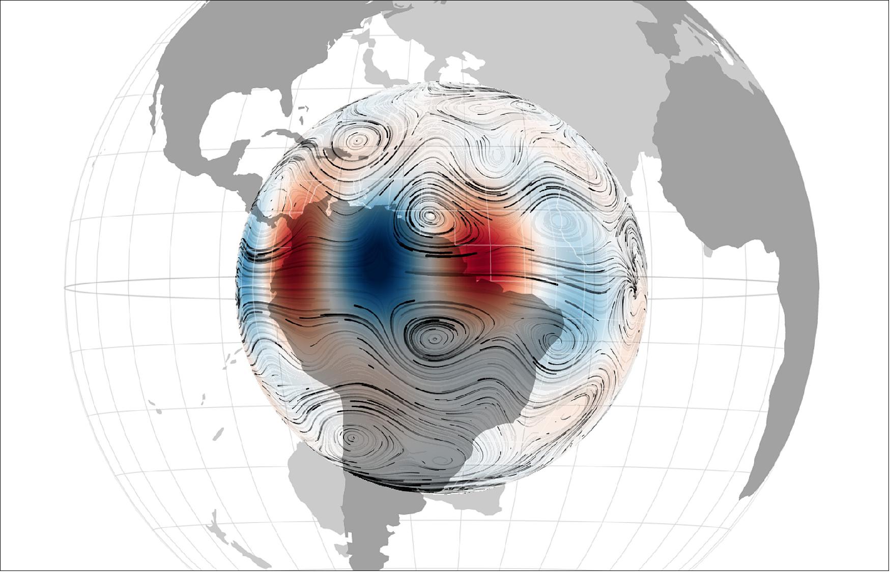
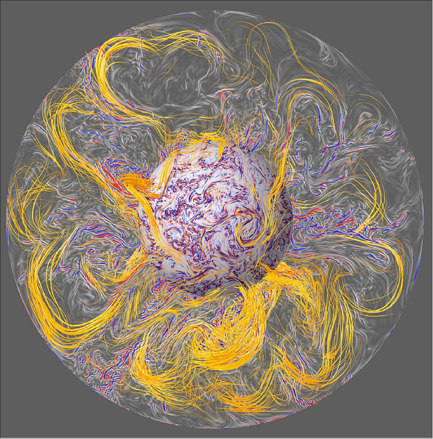
• May 23, 2022: Using data from ESA's Swarm satellite mission, scientists have discovered a new type of magnetic wave sweeping across Earth's outer core every seven years, shedding light on previously unknown dynamics deep beneath the planet's surface. This groundbreaking finding, presented at ESA's Living Planet Symposium, reveals insights into Earth's magnetic field generation and interaction with solar wind, contributing to a better understanding of space weather and aiding in the preparation for potential impacts on communication networks and satellites. The research, published in Proceedings of the National Academy of Sciences, highlights the importance of satellite measurements in probing Earth's core and offers avenues for further exploration into the planet's geodynamic processes. 58) 59)
Figure 34: Discovery of new type of magnetic wave sweeping across the outermost part of Earth's core, enabled by information collected by the Swarm satellite. (video credit: ESA/Planetary Visions)
• December 15, 2021: ESA's Cluster and Swarm missions, along with ground-based measurements, have confirmed a direct connection between bursty bulk flows in Earth's magnetosphere and abrupt changes in the magnetic field near the planet's surface. These changes can induce geomagnetically induced currents, posing risks to pipelines and power lines. This groundbreaking discovery, detailed in Geophysical Research Letters, highlights the significance of understanding space weather phenomena for safeguarding communication networks, navigation systems, and satellites critical for daily life. The extended missions of Cluster and Swarm have enabled scientists to delve deeper into Earth's magnetosphere, offering valuable insights into potential space weather hazards and informing the development of reliable mitigation strategies. 60)
Figure 37: Magnetic reconnection in Earth's magnetosphere. This animation shows the sequence of events that give rise to magnetic reconnection in Earth's magnetosphere and, subsequently, to bright aurorae close to Earth's polar regions. (video credit: ESA/ATG medialab)
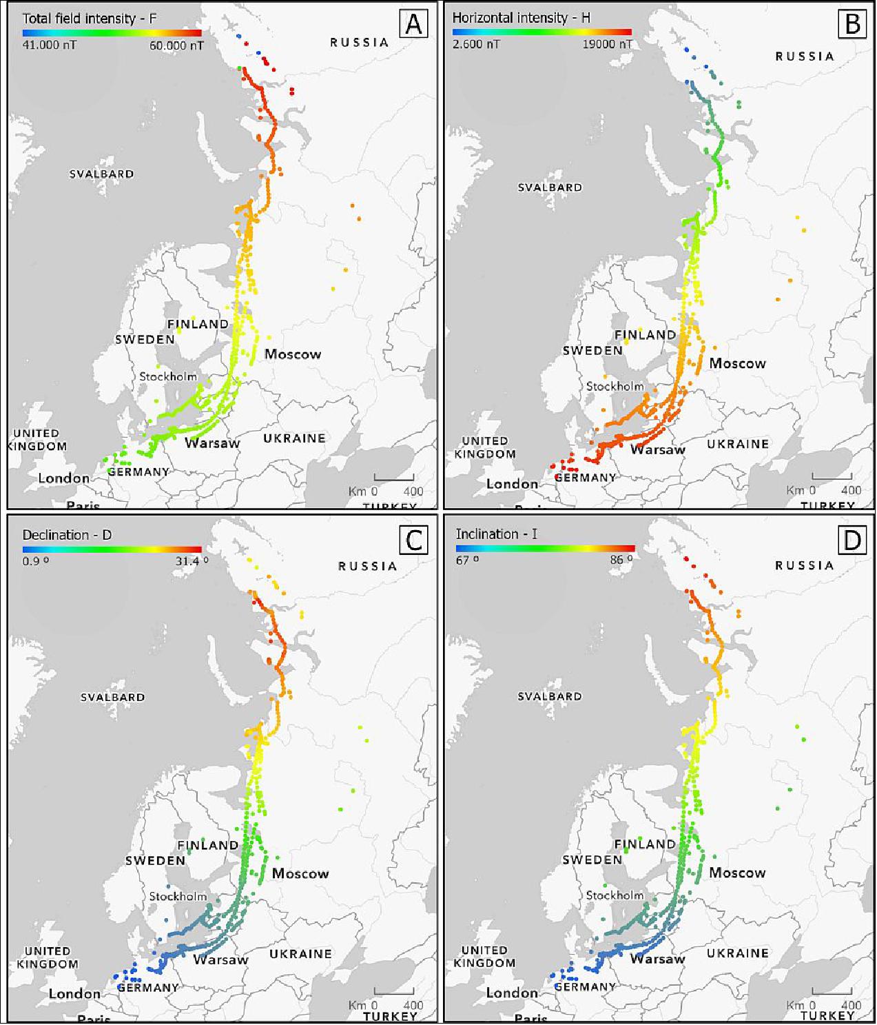
• July 9, 2021: Utilizing data from ESA's Swarm magnetic field mission, researchers have developed a novel tool to analyze the relationship between the Earth's magnetic field and the flight paths of migratory birds. This groundbreaking advancement, detailed in Movement Ecology, enables ecologists to assess the strength and direction of the magnetic field along animal migratory routes, shedding light on how animals navigate vast distances. By integrating Swarm data with animal tracking information from Movebank, this tool offers new insights into migration behavior and demonstrates the impact of geomagnetic storms on animal movement. 62) 63)
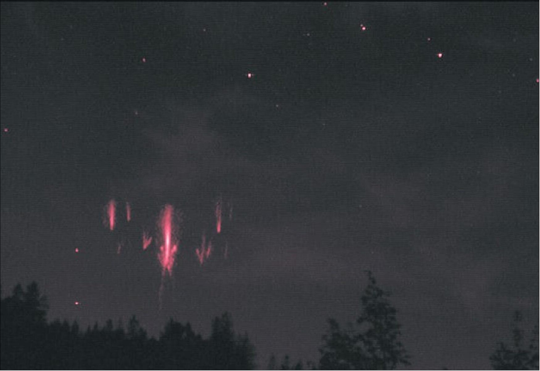
• May 18, 2021: A rare convergence of photographic evidence from a lightning enthusiast, measurements from ESA's Swarm satellite mission, and ground recordings have provided valuable insights into transient luminous events (TLEs), elusive types of lightning that shoot upwards into space. These TLEs, including sprites, jets, and elves, occur high in the atmosphere and are linked to electrical activity in thunderstorms. The coincidence of photographic evidence with Swarm's measurements aids in understanding how lightning propagates into the ionosphere, potentially influencing Earth's magnetic field, and highlights the significance of interdisciplinary collaboration in atmospheric research. 64)
• March 9, 2021: An international team of scientists has utilized magnetic data from ESA's Swarm satellite mission along with aeromagnetic data to uncover the geological secrets hidden beneath Antarctica's thick ice sheets, shedding light on the continent's tectonic history and its connection to neighboring landmasses like Australia, India, and South Africa. This groundbreaking research, published in Scientific Reports, merges satellite and airborne magnetic data to create a comprehensive picture of Antarctica's sub-ice geology, offering valuable insights into Earth's evolution and the dynamics of its least accessible continent. 66) 67)
• January 12, 2021: Using data from ESA's Swarm satellite constellation, scientists have uncovered a surprising revelation about the distribution of electromagnetic energy from the solar wind into Earth's atmosphere: more energy is directed towards the magnetic north pole than towards the magnetic south pole. This unexpected finding, published in Nature Communications, suggests that Earth's magnetic field not only shields us from solar radiation but also actively controls the distribution of energy into the upper atmosphere. Lead author Ivan Pakhotin explains that the asymmetry in energy distribution could lead to differences in space weather effects and atmospheric chemistry between the northern and southern hemispheres. These insights, made possible by Swarm's data, are crucial for understanding space weather dynamics and enhancing early warning systems to mitigate potential impacts on modern infrastructure. 68) 69)
• August 17, 2020: The South Atlantic Anomaly (SAA) represents a weakened area in Earth's magnetic field over South America and the southern Atlantic Ocean, allowing charged particles from the Sun to dip closer to the surface. NASA scientists are closely monitoring this anomaly due to its potential to disrupt satellite operations as particles can interfere with onboard computers. The anomaly, stemming from the dynamics of Earth's molten core and the tilt of its magnetic axis, is expanding and splitting, posing challenges for satellite missions. Scientists use observations and physics to model the SAA's changes and contribute to global forecasts of Earth's magnetic field, crucial for understanding the planet's evolving dynamics and ensuring satellite safety. 70)
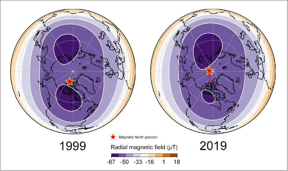
• May 20, 2020: The South Atlantic Anomaly (SAA), a weakening area in Earth's magnetic field stretching from Africa to South America, is perplexing geophysicists and causing technical disturbances in satellites. Over the last 50 years, the SAA has expanded and intensified, with its minimum field strength decreasing and a second center of minimum intensity emerging southwest of Africa. Utilizing data from ESA's Swarm satellite constellation, scientists are striving to comprehend the anomaly's development and its underlying processes within Earth's core. While speculation about an impending pole reversal exists, the SAA's current fluctuations remain within normal levels, albeit posing challenges for satellite operations due to increased exposure to charged particles. 71)
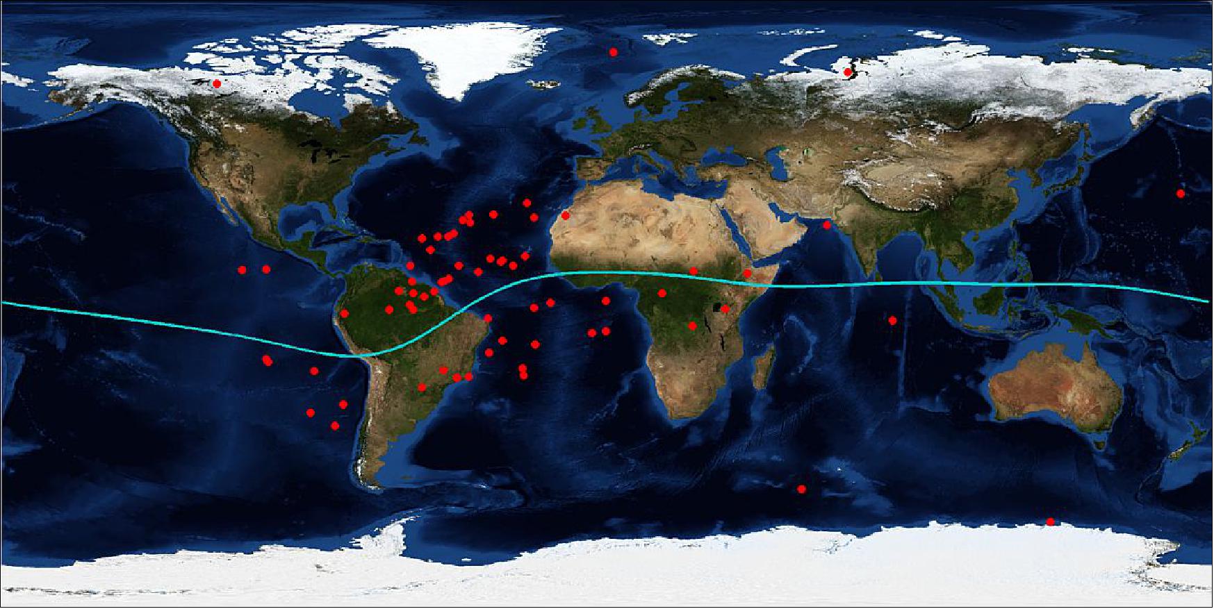
Figure 45: White dots on the map indicate individual events when Swarm instruments registered the impact of radiation from April 2014 to August 2019. The background is the magnetic field strength at the satellite altitude of 450 km (video credit: Division of Geomagnetism, DTU Space)
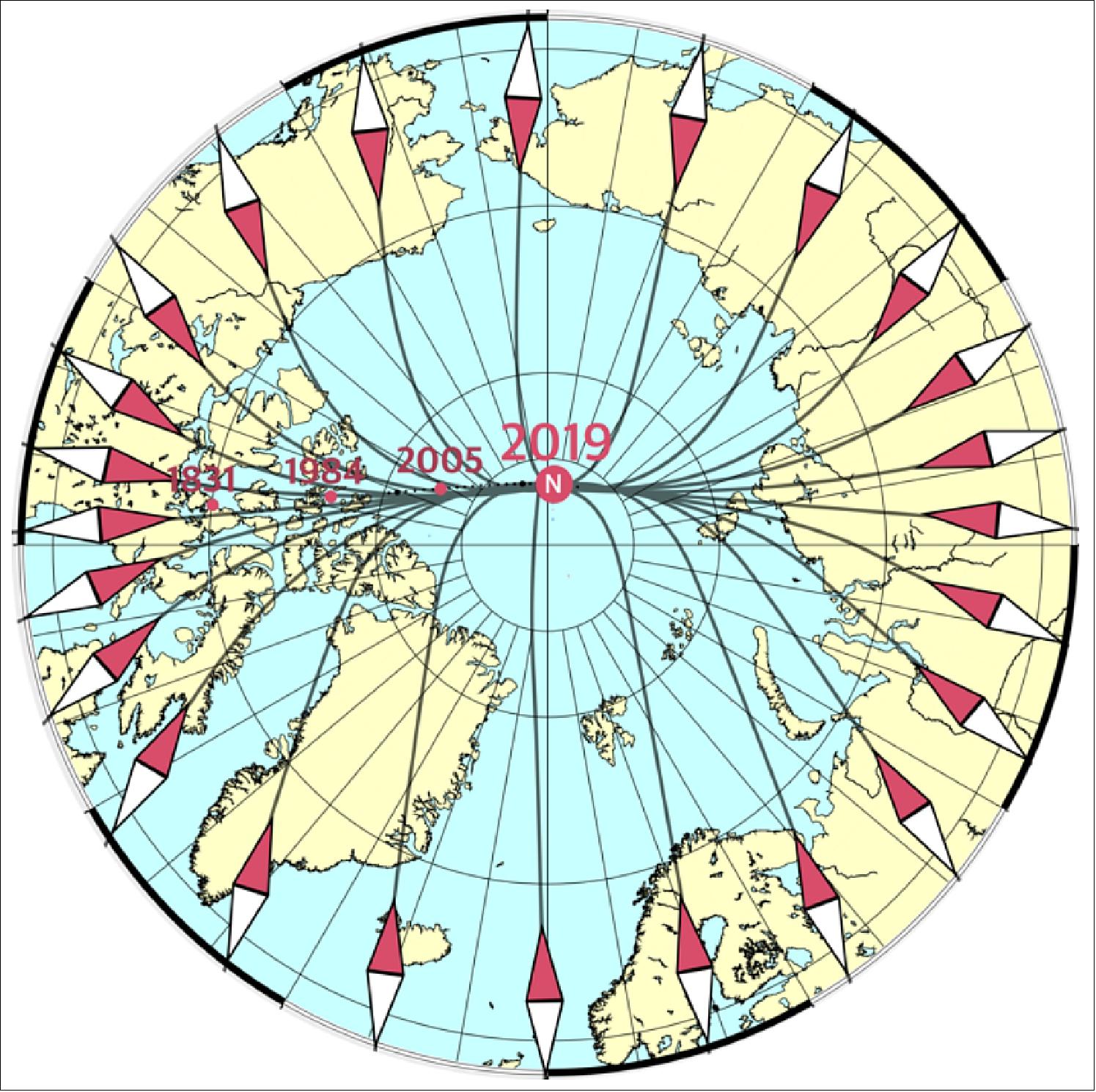
• May 14, 2020: Scientists have long observed the north magnetic pole's gradual movement, but since the 1990s, it has accelerated significantly, now racing towards Siberia at a speed of 50-60 km per year. Thanks to data from ESA's Swarm satellite mission, researchers have linked this phenomenon to changes in the circulation pattern of the Earth's core beneath Canada. This shift has weakened the magnetic field patch under Canada, causing the pole to drift eastward. While models predict the pole's continued movement towards Siberia in the coming decades, even small adjustments in the core's magnetic field could potentially redirect its trajectory back towards Canada. 72)
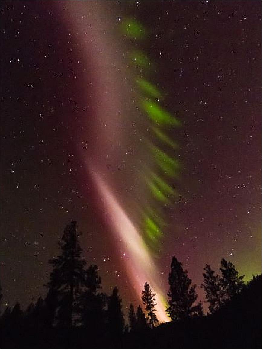
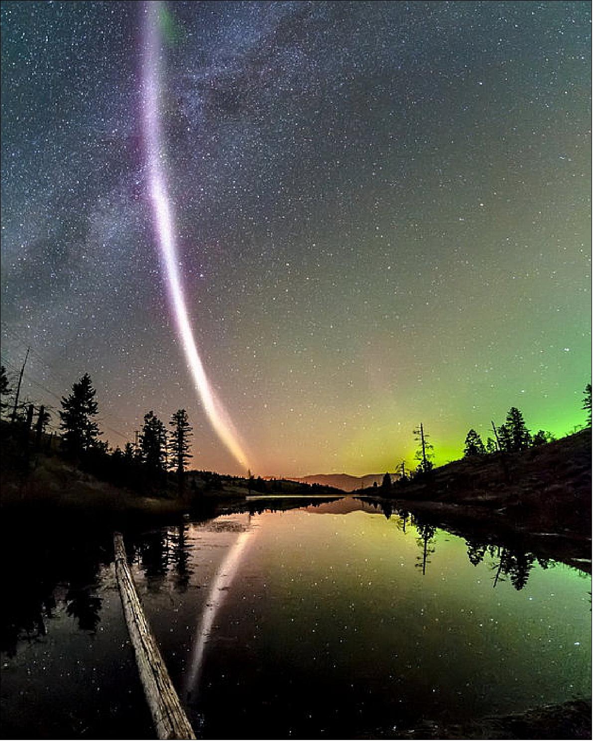
• November 27, 2019: Discovered by citizen scientists in 2017, the mysterious purple streaks of light in the sky known as Steve, accompanied by green "picket fences," have intrigued researchers. Using data from ESA's Swarm mission and photographs from the Alberta Aurora Chasers, scientists have determined that Steve comprises fast-moving streams of hot atomic particles, distinct from typical auroras caused by energetic electrons. Through triangulation of photographs and identification of stars in the background, they estimated Steve's altitude range to be 130 to 270 km, while the picket fence ranges from 95 to 150 km. Additionally, alignment along magnetic field lines suggests a deeper connection between the two phenomena, aiding in unraveling the enigma surrounding Steve. 73)

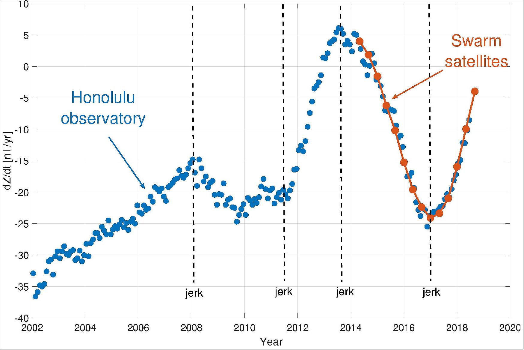
• May 1, 2019: Geomagnetic jerks, sudden and unpredictable accelerations in Earth's magnetic field, have puzzled scientists since their discovery in 1978. Recent research, utilizing data from ground-based observatories and ESA's Swarm satellites, has shed light on these phenomena, revealing that they occur globally approximately every three to 12 years and are driven by rapid hydromagnetic waves originating within Earth's core. These waves, interacting with slow convection movements, cause sharp changes in the flow of liquid beneath the magnetic field, resulting in geomagnetic jerks. Understanding these jerks is crucial for forecasting changes in the magnetic field, which protects Earth from solar storms and is vital for various modern technologies. 75) 76)
• April 25, 2019: STEVE, a celestial phenomenon distinct from typical auroras, has captured attention for its unique appearance of pinkish-red ribbons and green picket fence columns in the night sky. Recent research suggests that STEVE is caused by a combination of mechanisms involving heating of charged particles in Earth's atmosphere and energetic electrons, contrasting with the charged particle precipitation that powers auroras. While the picket fence phenomenon aligns with typical auroral processes, the mauve streaks of STEVE result from particle heating without precipitation. Analyzing satellite data and ground images, scientists determined that STEVE originates from a flowing river of charged particles colliding in Earth's ionosphere, emitting light akin to incandescent light bulbs. Moreover, the study found that the picket fence occurs simultaneously in both hemispheres, driven by energetic electrons energized by high-frequency waves from Earth's magnetosphere. The involvement of citizen scientists in STEVE research has been pivotal, providing valuable ground-based images and data for analysis, highlighting the role of public engagement in advancing scientific understanding. 77)
• February 8, 2019: The magnetic north pole's accelerated movement, currently at a rate of about 55 km per year, has necessitated an urgent update to the World Magnetic Model, crucial for navigation systems like smartphones and Google Maps. Traditionally, the model undergoes revisions every five years, but the rapid shift prompted an out-of-cycle update, facilitated in part by data from ESA's Swarm mission. Since its launch in 2013, the Swarm constellation has been monitoring Earth's magnetic field variations, including the position of the magnetic north pole, providing essential information for billions of users relying on navigation systems in their daily lives, unbeknownst to many. 78)
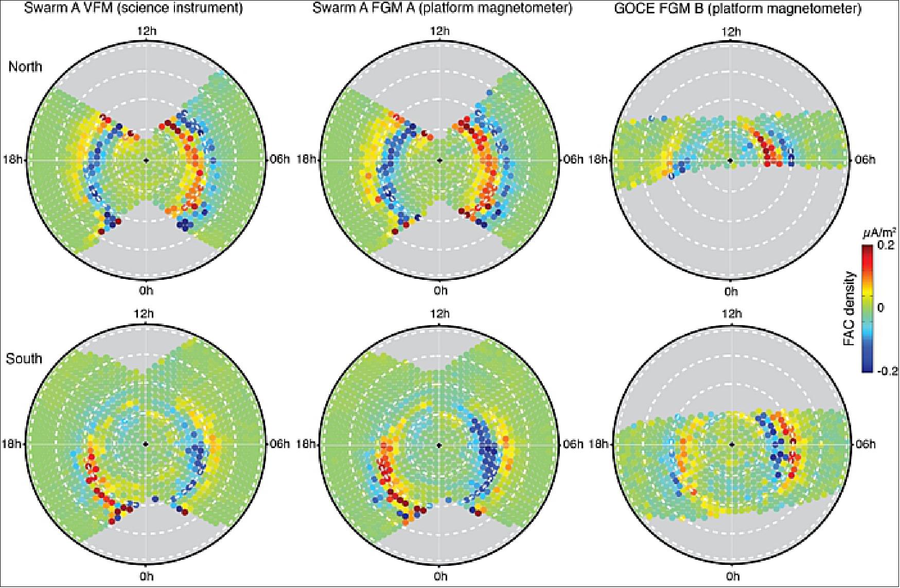
• November 7, 2018: Researchers have explored the potential of utilizing platform magnetometers, typically employed for satellite orientation, to monitor space weather impacts on Earth's magnetic field. Investigating data from ESA's Swarm, GOCE, and LISA Pathfinder missions, they compared platform magnetometer readings with scientific magnetometer data, concluding that the former can offer valuable insights into space weather phenomena. This cost-effective approach could be further enhanced through advanced data processing techniques, potentially expanding access to crucial space weather monitoring capabilities beyond engineering circles. 79)
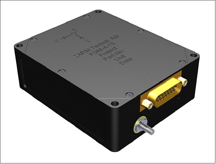
• June 28, 2018: A team of researchers, supported by ESA's Basic Activities, has explored a novel method of monitoring space weather by analyzing data from spacecraft platform magnetometers typically used for attitude control. These magnetometers, designed to keep spacecraft oriented correctly, were investigated for their potential to monitor the impact of solar storms on Earth's magnetic field. Through the analysis of data from missions such as Swarm, GOCE, and LISA Pathfinder, the team demonstrated that platform magnetometers can provide valuable insights into space weather phenomena, offering a cost-effective approach to enhancing space weather monitoring capabilities. Their findings suggest the feasibility of leveraging existing spacecraft instrumentation to improve our understanding of space weather and its potential effects on critical infrastructure. 80)
• April 13, 2018: ESA's Swarm mission has recently unveiled a trove of groundbreaking findings at the European Geosciences Union meeting in Vienna, Austria. Among these discoveries, Swarm has provided unexpected insights into lightning in the upper atmosphere and geomagnetic storms. By temporarily running its magnetometers in a higher frequency mode, Swarm captured some 4000 instances of lightning-induced electromagnetic waves, known as whistlers, in just four days, offering a unique opportunity to study the ionosphere and the propagation of lightning signals into space. The whoosh of these lightning whistlers can be heard in the animation of Figure 57. Additionally, Swarm's observations have shed light on the development of storms in the upper atmosphere during geomagnetic events, revealing a massive movement of gas triggered by Joule heating, thus enhancing our understanding of Earth's magnetic field and its interactions with space (Figure 58). 81) 82)
Figure 57: Whoosh of the lightning whistlers. (image credit: Institut de Physique du Globe de Paris)
Figure 58: St. Parick's day storm of 17 March 2015. (video credit: ESA)
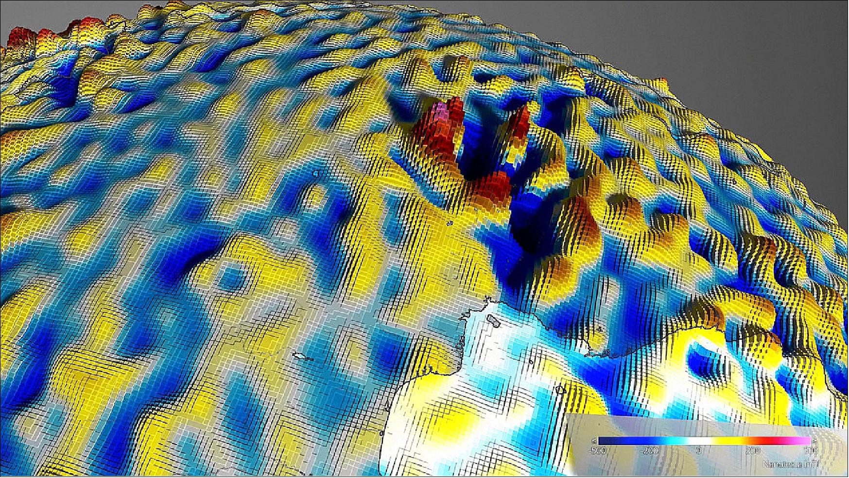
• April 10, 2018: ESA's Swarm satellites, along with historical data from the German CHAMP satellite and observations from ships and aircraft, have generated the most detailed map to date of the tiny magnetic signals produced by Earth's lithosphere, shown in Figure 59. Led by Erwan Thebault from the University of Nantes in France, this high-resolution model, with a scale of 250 km, provides unprecedented insights into the geological structures of Earth's crust. By combining satellite measurements with near-surface observations, particularly beneath Australia where aircraft measurements have achieved a resolution of 50 km, scientists have gained a new understanding of the lithosphere's magnetic field, shedding light on Earth's magnetic history and the movement of tectonic plates over millions of years. 85) 86)
Figure 59: Video map of tiny magnetic signals generated by Earth’s lithosphere, constructed with the measurements collected by the three Swarm satellites over four years, as well as with historical data from the German CHAMP satellite. (image credit: ESA/Planetary Visions)
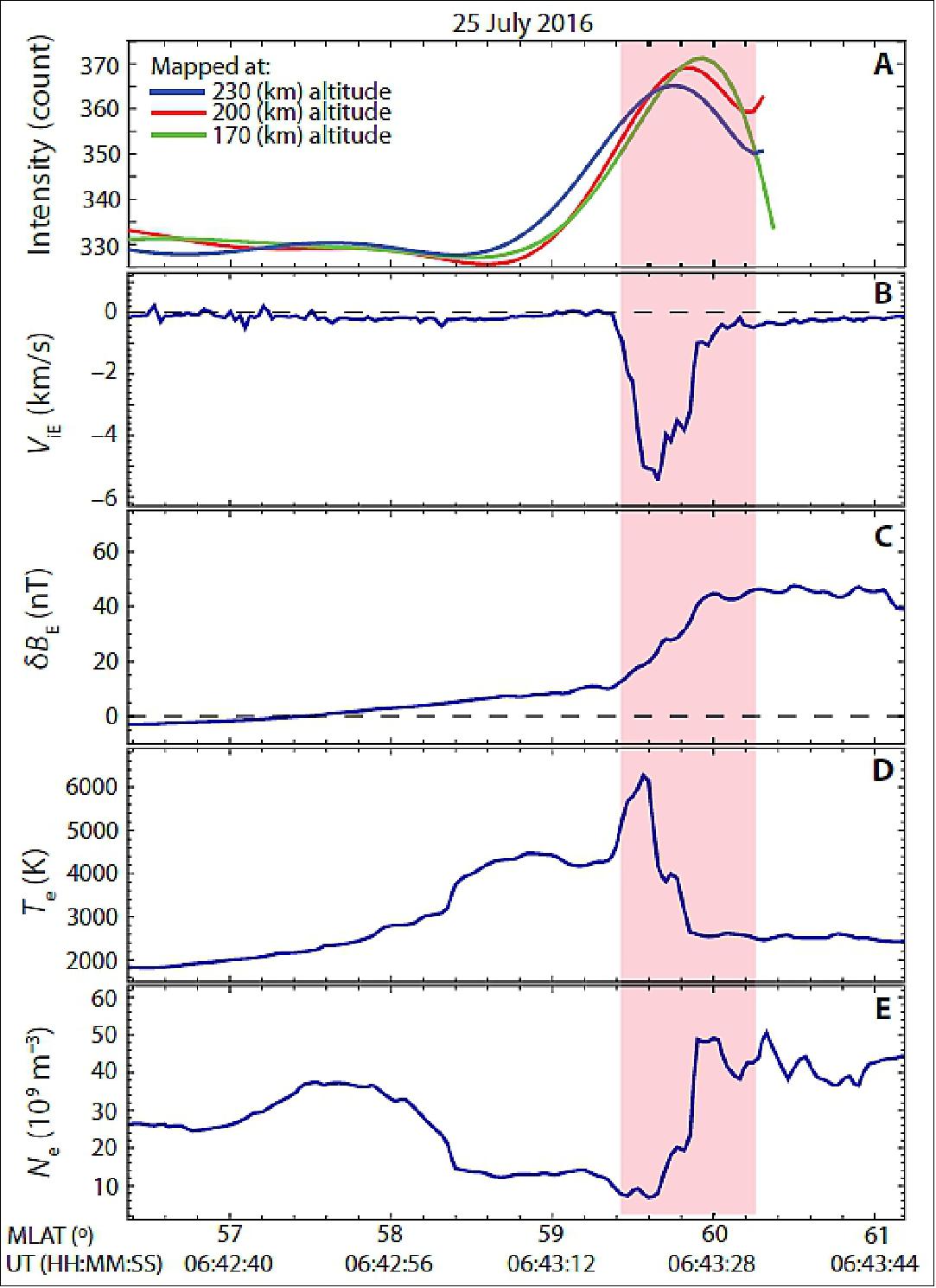
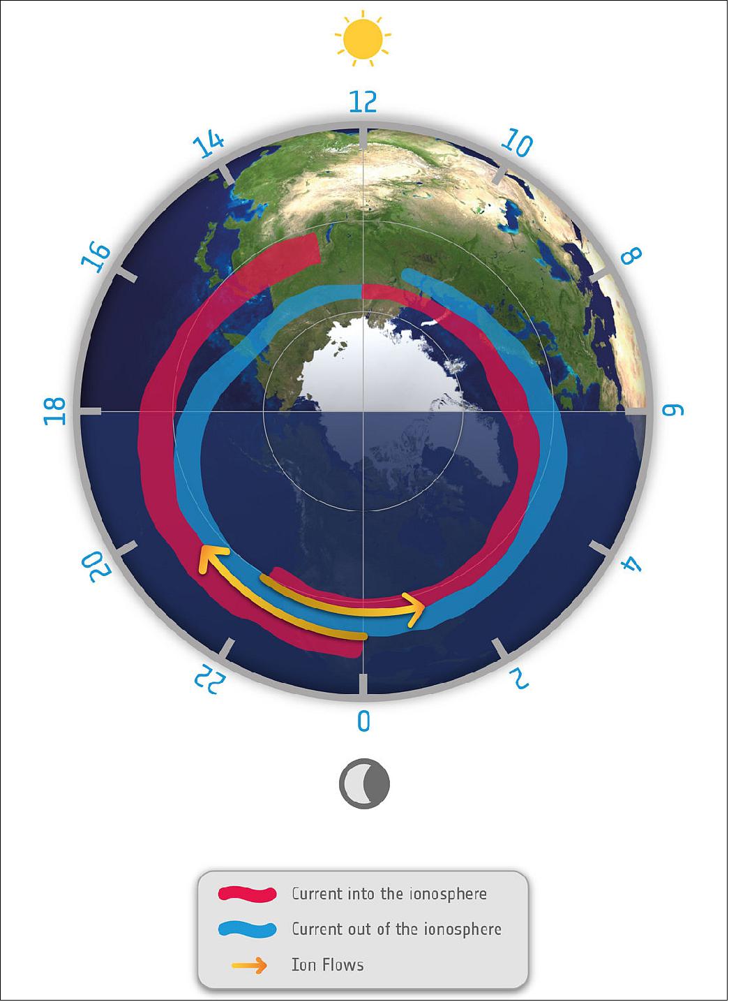
• March 16, 2018: Discovered in 2016 and dubbed "Steve," this peculiar auroral phenomenon has intrigued scientists and amateur skywatchers alike. Initially identified by members of the Aurora Chasers Facebook group, Steve presents as a narrow purple band accompanied by unstable green features resembling a picket fence, moving westward. Thanks to data from ESA's Swarm mission and ground observations, researchers led by Elizabeth MacDonald have shed light on Steve's nature. It was found that Steve represents an optical auroral phenomenon, characterized by a clear westward ion flow reaching speeds of up to 5.5 km/s, accompanied by an increase in eastward magnetic field perturbation and elevated electron temperatures. These findings offer unprecedented insights into the dynamics of auroral phenomena and ionospheric processes. 87) 88) 89) 90) 91)
- Figure 60 presents detailed observations and measurements related to the STEVE (Strong Thermal Emission Velocity Enhancement) phenomenon. Plot A illustrates the intensity of the STEVE arc along the trajectory of the Swarm A satellite, indicating its location just below 60º magnetic latitude across various emission heights. Plot B depicts ion velocity data, showing a pronounced westward flow during peak STEVE optical emission. Plot C shows a positive gradient in magnetic field perturbation, corresponding to a small downward Field-Aligned Current (FAC). Plots D and E display data from the Langmuir probe, revealing an elevated electron temperature and minimum electron density within the region of the arc, with distinct variations in electron density on both the equatorward and poleward sides.
• February 22, 2018: ESA and Canada have collaborated to integrate Canada's Cassiope satellite, specifically its e-POP instrument package, into ESA's Swarm mission, effectively turning Swarm into a four-satellite mission. This collaboration aims to enhance the understanding of space weather and phenomena like the aurora borealis by leveraging the complementary measurement capabilities of both missions. The integration formalized through ESA's Third Party Mission program enhances the scientific potential of the Swarm mission, allowing for new investigations into magnetosphere-ionosphere coupling, Earth's magnetic field, upper atmospheric dynamics, and aurora dynamics. This partnership underscores the value of international cooperation in advancing scientific understanding and data accessibility in space research. 92)
• February 15, 2018: The Swarm mission has provided unprecedented insights into the intricate relationship between Earth and the Sun, revealing the complex dynamics of the exchange of energy and charged particles between the magnetosphere and ionosphere. By studying field-aligned currents at different spatial scales, Swarm has challenged previous assumptions, showing that smaller currents can carry significant energy and have a complex relationship with larger currents. These findings not only deepen our understanding of Earth's response to solar activity but also have practical implications for navigation, telecommunication systems, and preparedness for solar storms. As Swarm continues to unveil new discoveries, it becomes increasingly integral to understanding the fundamental processes that govern our planet's interaction with the Sun. 93) 94)
- The shimmering green and purple light displays of the auroras in the skies above the polar regions are a visible manifestation of energy and particles travelling along magnetic field lines (Figure 62).

• June 2017: The presentations of the Fourth Swarm Science Meeting, Banff, Alberta, Canada, 20-24 March 2107 are available at http://esaconferencebureau.com/2017-events/17c04/presentations 97)
• April 21, 2017: The discovery of a mysterious purple ribbon of light in the night sky, affectionately named "Steve" by citizen scientists, has been facilitated by social media platforms and ground-based observations. With the aid of ESA's Swarm mission data and a network of all-sky cameras, researchers have begun to unravel the nature of this phenomenon. Steve, characterized by its significant temperature increase and fast-flowing gas ribbon, represents a previously unnoticed but surprisingly common occurrence, highlighting the importance of collaboration between scientists and citizen scientists in advancing our understanding of Earth's magnetic field interactions with the solar wind. 98)
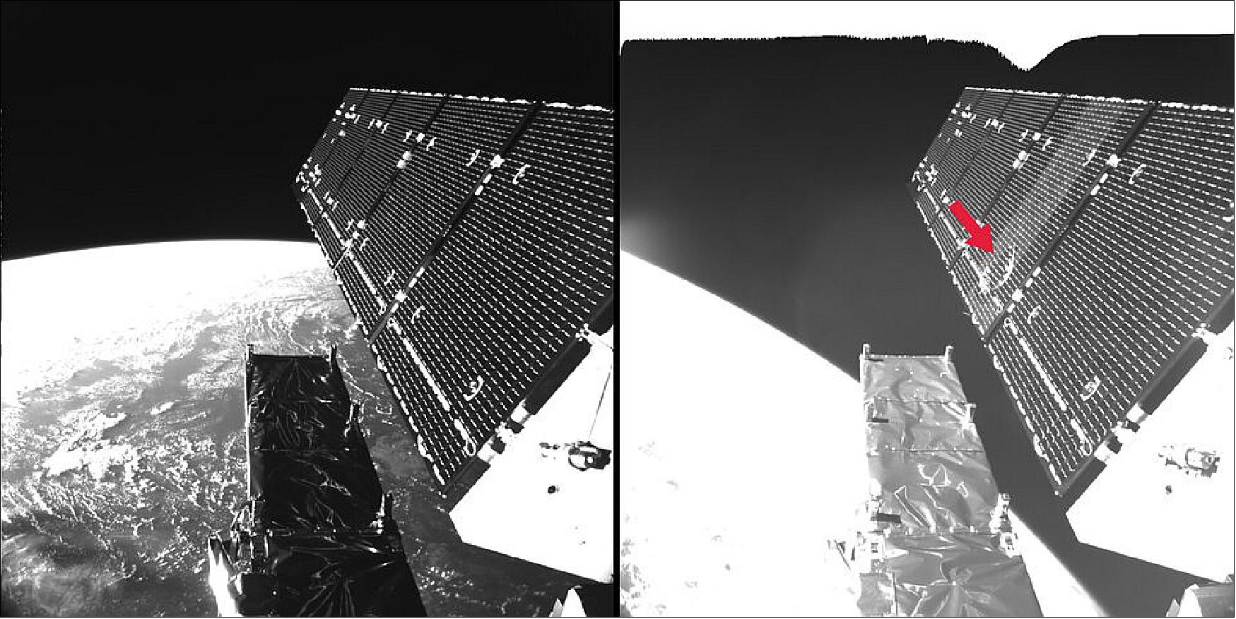
• March 2017: The Swarm mission's three platforms are operating smoothly, with effective control by a shared team also managing ESA Earth-Explorer missions. While payload operations have proven more complex and resource-intensive than anticipated, ongoing testing and fine-tuning activities, particularly for the Electrical Field Instrument (EFI), remain a continuous challenge. Plans for a mission extension are underway, with the Ground Segment deemed capable of supporting it, although technical and budgetary considerations are being assessed. Additionally, efforts to understand image quality degradation and implement improvements have been extensive across all satellites. 99)
• March 23, 2017: Scientists from the University of Calgary, presenting at the Swarm Science Meeting, revealed groundbreaking discoveries facilitated by ESA's Swarm mission data. Utilizing measurements from the Swarm satellites, they unveiled supersonic plasma jets, dubbed 'Birkeland current boundary flows', driven by strong electric fields in the upper atmosphere. These jets, marking the boundary between opposing current sheets, reach temperatures nearing 10,000°C, alter the ionosphere's chemical composition, and induce upward flows that can lead to atmospheric material loss into space. This finding enhances understanding of the Birkeland current circuit, a key component of Earth's magnetosphere-ionosphere system, demonstrating the pivotal role of Swarm in unraveling the complexities of our planet's atmospheric dynamics. 100)
• March 22, 2017: The Swarm mission, through magnetic field measurements, has uncovered significant variations in the seasonal behavior of Birkeland currents in the polar regions, differing between the northern and southern hemispheres. These findings, presented at the Swarm science meeting, reveal insights into the interplay between Earth's magnetic field and the solar wind, shedding light on how solar wind orientation influences the strength of Birkeland currents and their connection to Earth's magnetic field. The research highlights asymmetries in Earth's main magnetic field as a key factor driving hemispheric differences in current strength, offering valuable insights into the complex dynamics of Earth's magnetosphere-ionosphere system. 101)
• March 21, 2017: ESA's Swarm satellites have achieved a significant breakthrough in mapping Earth's lithospheric magnetic field, which is notoriously challenging to detect from space due to its weakness. By combining Swarm data with historical measurements from the CHAMP satellite and employing advanced modeling techniques, researchers have produced the highest-resolution map to date of the magnetic signals emanating from Earth's crust. This new map, presented at the Swarm Science Meeting, reveals detailed variations in the magnetic field caused by geological structures, offering insights into Earth's magnetic history and crustal composition. Anomalies such as the sharp and strong magnetic field observed in Central African Republic suggest potential geological events like meteorite impacts millions of years ago, underscoring the value of satellite-based observations in understanding Earth's complex magnetic structure (Figure 101). 102)
• February 1, 2017: ESA's Swarm mission recently faced a potential collision with space debris, prompting a meticulously orchestrated response to ensure the safety of Swarm-B. The threat arose when a piece of debris from the Cosmos 375 satellite was projected to come dangerously close to Swarm-B's orbit. Swift action ensued, involving collaboration among various teams to plan a debris avoidance maneuver. However, updated tracking data and precise GPS measurements ultimately revealed that the risk of collision fell below acceptable thresholds, allowing mission managers to confidently abort the maneuver and resume normal operations. This incident underscores the increasing risk posed by space debris and highlights the importance of vigilant monitoring and proactive measures to safeguard spacecraft in orbit. 103)
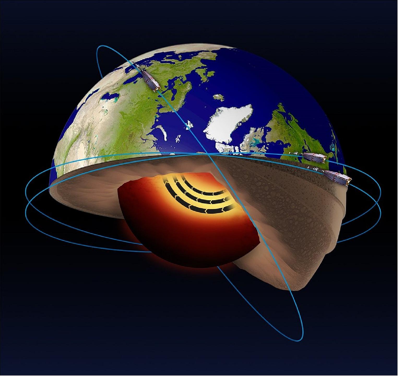
• December 19, 2016: ESA's Swarm mission, launched in 2013, has revealed a previously unknown jet stream deep within Earth's core, thanks to its precise measurements of the planet's magnetic field. This discovery, described in a recent paper in Nature Geoscience, highlights the mission's capability to untangle the complex magnetic fields originating from various layers of Earth's interior. The jet stream, observed for the first time, is found to be moving at remarkable speeds, three times faster than typical outer-core velocities, and its existence sheds light on the dynamic processes occurring within Earth's core. Scientists believe that changes in the magnetic field within the core may play a role in accelerating the jet stream, and further research enabled by Swarm's high-resolution measurements promises more revelations about our planet's hidden depths. 104) 105)
• October 28, 2016: ESA's Swarm mission has uncovered the cause behind intermittent GPS signal losses experienced by low-orbiting satellites, revealing a connection to Equatorial Plasma Irregularities (EPIs) in the ionosphere, termed "ionospheric thunderstorms." These EPIs, characterized by rapid changes in electron density in the F region of the ionosphere, predominantly occur near Earth's magnetic equator and coincide with GPS signal disruptions, particularly in low-latitude regions. The study, utilizing Swarm's high-resolution GPS measurements, identified a distinct correlation between EPIs and loss of GPS signal, with potential implications for improving future GPS systems and enhancing our understanding of upper-atmosphere dynamics. 106) 107)
• October 3, 2016: ESA's Swarm satellites have made groundbreaking discoveries regarding the Earth's magnetic field, uncovering the subtle magnetic contribution of ocean tides and using this data to unveil the electrical properties of the Earth's upper mantle. Through precise measurements, Swarm, along with data from the Champ mission, has enabled scientists to differentiate between the rigid lithosphere and the more fluid asthenosphere beneath, shedding light on plate tectonics and conductivity variations. This pioneering research offers valuable insights into Earth's interior structure and functioning, providing a deeper understanding of our planet as a whole system. 108) 109) 110)
• August 2016: Since overcoming initial challenges during commissioning, the Swarm satellite constellation has been operating smoothly, with all platforms functioning as expected and few anomalies reported. A key focus has been refining error-handling strategies for the Mass Memory Unit (MMU), distinguishing between Single Event Functional Interruptions (SEFI) and Single Stuck Bits (SSB) to optimize memory management. This new approach aims to minimize unnecessary MMU resets, which previously resulted in data loss. Additionally, efforts have been made to enhance the performance of the GPS receivers (GPSR) through software updates, including expanding the field-of-view to 88º to improve tracking capabilities and scientific data collection. (Ref. 160)
Parameter | SWA (Swarm-A) | SWB (Swarm-B) | SWC (Swarm-C) |
SEFI (Single Event Functional Interruptions) | 6 | 6 | 15 |
SSB (Single Stuck Bit) | 1 | 41 | 1 |
• August 2016: Since the completion of the orbit acquisition phase in April 2014, the Swarm satellite constellation has operated with Swarm-B in a higher orbit with an inclination of 87.8º and an altitude gradually decreasing from 520 km, while Swarm-A and Swarm-C form the lower pair at an initial altitude of 473 km and an inclination of 87.4º. Originally, the lower pair was expected to decay to 300 km altitude within four years after launch, but due to lower-than-expected solar activity and geomagnetic forces, the decay process has been slower than anticipated. To mitigate this, adjustments were made to reduce the inclination difference between Swarm-B and Swarm-A/C, minimizing the drift between their orbit planes to 1.5 hours per year to ensure alignment throughout the mission duration. 111)
• May 10, 2016: ESA's Swarm satellite trio, launched in late 2013, has been instrumental in mapping changes in Earth's magnetic field with unprecedented detail. These measurements reveal fluctuations in field strength, indicating a 3.5% weakening over North America and a 2% strengthening over Asia, while also tracking the movement of the magnetic north pole towards Asia and the westward drift of the South Atlantic Anomaly. Moreover, Swarm data highlight rapid localized field changes, suggesting accelerations in liquid metal flow within the core. These findings underscore the mission's significance in enhancing our understanding of Earth's magnetic field dynamics and their broader implications for natural processes and space weather. 112)
• December 22, 2015: The Swarm team has released an ASM-VFM Residual dataset, now accessible in the "Advanced" folder of the ESA FTP server. This dataset spans from the start of the mission until July 17, 2015, covering all Swarm spacecraft. It is designed for investigating the scalar residuals between the readings of the scalar magnetometer (ASM) and the vector magnetometer (VFM). 114)
• July 2015: The Swarm mission is experiencing high scientific productivity across various areas, from the deep interior of Earth's outer core to the outermost layers of the thermosphere and magnetosphere. The constellation approach has proven instrumental in unraveling and distinguishing the various contributors to the magnetic and electric field measurements. Activities to maintain the constellation are progressing well, especially in optimizing the operation of the lower pair of satellites for magnetic field gradient measurements. The release of the first official geophysical models and ongoing efforts in calibration/validation indicate continuous improvement in data quality and further advancement in mission objectives. 115)
• June 22, 2015: After one and a half years in orbit, the Swarm satellites have provided valuable insights into Earth's interior and the dynamics of the upper atmosphere, ranging from the ionosphere to the outer layers of the magnetic shield. Recent scientific papers published in Geophysical Research Letters highlight the mission's significant potential, confirming the success of the meticulous efforts invested in making Swarm a groundbreaking magnetometry mission. Rune Floberghagen, ESA's Swarm Mission Manager, emphasized the rewarding outcome of these efforts, while Nils Olsen, leading the Swarm Satellite Constellation Application and Research Facility, emphasized the importance of ensuring accessibility to the mission's initial results for the scientific community. 116) 117) 118) 119) 120)
• May 2015: Swarm's mission operations are ongoing, maintaining the satellite constellation to ensure optimal data collection for understanding Earth's magnetic field. Last year, early data from the mission were utilized to generate candidate solutions for the 2015 International Geomagnetic Reference Field (IGRF) model, a crucial update used across various applications and services dependent on geomagnetic data. This final model, IGRF-12, integrates Swarm data with historical satellite and ground-based observatory data. Additionally, Swarm has produced a detailed Initial Field Model, incorporating high-resolution crustal magnetic field computations, which has been made accessible to the scientific community. 121) 122)
• November 22, 2014: After a year in orbit, the Swarm constellation continues to gather high-quality scientific data through its seven identical instruments onboard. Recent reprocessing of early mission data aimed to support the development of candidate solutions for the 2015 International Geomagnetic Reference Field (IGRF) model, with various Swarm science team members contributing to these models using data from both types of magnetometers. The IGRF model, updated every five years, serves as a crucial reference for numerous applications and services reliant on geomagnetic data. 123) 124)
• October 2014: The Swarm Absolute Scalar Magnetometer (ASM) instruments, operational on the three Swarm satellites since November 26, 2013, have provided early results confirming the achievement of initial mission goals. Operating continuously except for specific operational periods, the ASM instruments have demonstrated low noise levels and a clean electromagnetic environment, enabling the detection of tiny magnetic field signals. The ASM scalar data exhibits exceptional performance, offering precise and consistent measurements, essential for studying subtle magnetic field variations.
- Additionally, the ASM's ability to function simultaneously as both an absolute scalar magnetometer and a vector field magnetometer has been validated, presenting a world-first capability. Furthermore, the ASM's vector mode data show scientific promise and may become an official product of the Swarm mission. Despite a malfunction in the redundant ASM model on Swarm Charlie, the nominal model's operational success on all three satellites ensures minimal impact on the mission's objectives. Early functional verifications and subsequent detailed assessments of ASM performance have been conducted, setting the stage for continued utilization of this innovative instrument. 125)
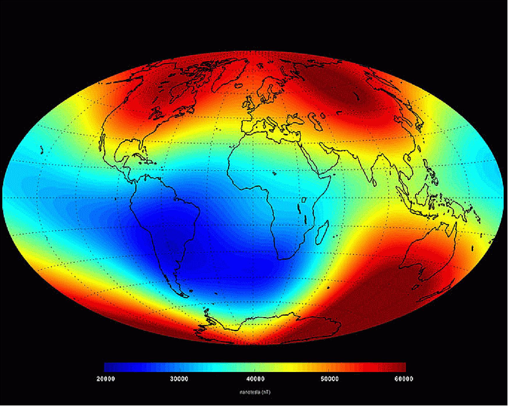
• June 19, 2014: ESA's Swarm constellation, launched in November 2013, has begun unveiling the latest changes in Earth's magnetic field, crucial for shielding the planet from cosmic radiation and charged particles. Recent measurements over six months highlight a general trend of field weakening, particularly pronounced over the Western Hemisphere, alongside unexpected strengthening in regions like the southern Indian Ocean. Additionally, the magnetic North's shift towards Siberia is confirmed. These observations, primarily stemming from Earth's core, will undergo further analysis to discern contributions from other sources like the mantle, crust, oceans, ionosphere, and magnetosphere. Insights gained will elucidate various natural processes and space weather phenomena, offering a deeper comprehension of the magnetic field's weakening, notably prominent over the South Atlantic Ocean, known as the South Atlantic Anomaly, where satellite disruptions occur due to radiation exposure. 126) 127)
• May 7, 2014: ESA's Swarm satellites, operational for only five months, have already surpassed the precision achieved by previous missions after a decade. Engineers completed the commissioning phase and initiated operations Phase-E2 in April 2014, achieving the final orbital constellation by mid-April. Tasked with unraveling Earth's magnetic field mysteries, Swarm meticulously measures and disentangles magnetic readings from various sources, including the core, mantle, crust, oceans, ionosphere, and magnetosphere. Additionally, it provides data for calculating the electric field near each satellite, crucial for upper atmosphere studies. With two satellites orbiting side by side at 462 km and the third at 510 km, Swarm's readings aid in distinguishing solar activity-induced magnetic field changes from those originating within Earth. Despite being in the fine-tuning phase, Swarm has already provided sufficient data to construct magnetic field models, demonstrating its remarkable efficiency in a short timeframe. Access to the mission's magnetic field data will be granted to scientists in the coming weeks. 128) 129)
• February 2014: Since the launch of the Swarm constellation last November, engineers have been diligently conducting a commissioning phase to ensure the proper functioning of the satellites and instruments. This crucial phase precedes the mission's data collection, which aims to enhance our comprehension of Earth's intricate and ever-changing magnetic field. Tricky maneuvers are ongoing to position the Swarm satellites in their designated orbits for optimal data acquisition. Due to lower-than-expected solar activity, adjustments to the original orbit placement plan have been made based on input from the scientific community and ESA experts, leveraging insights from past missions like GOCE to navigate the effects of reduced atmospheric drag. 130)
• November 26, 2013: The Swarm satellites successfully completed the critical initial phase of their mission, known as the Launch and Early Orbit Phase (LEOP). Following their separation from the launcher, the satellites promptly initiated communication with Earth, marking the commencement of LEOP. Within 95 minutes of separation, signals from all three Swarm satellites were received, officially initiating the LEOP phase. Shortly thereafter, each satellite deployed its 4-meter-long boom containing essential scientific instruments. LEOP was officially concluded on November 24, 2013, confirming the successful transition to the next phase of the mission. 131)
Sensor Complement
High-precision and high-resolution measurements of the strength, direction and variation of the magnetic field, complemented by precise navigation, accelerometer and electric field measurements, will provide the necessary observations that are required to separate and model various sources of the geomagnetic field. 132) 133)
The observation concept is mainly determined by the following drivers set by the scientific payload: Each of the satellites carries an identical payload:
• High magnetic cleanliness required by the magnetometers (sub nT-range for VFM and ASM)
• EFI (Electrical Field Instrument) requires in-flight pointing with control accuracy of 5º
• ACC (Accelerometer) requires precise and stable accommodation in CoG (Center of Gravity).
Magnetic Field (all values 2σ) | - In-Situ magnitude with a random error < 0.3 nT |
Attitude knowledge | better than 0.1º |
Satellite position | - POD (Precise Orbit Determination) < 10 cm (rms) – L2 products |
Air drag (all values 2σ) | Vector components with a random error < 5 x 10⁻⁸ ms-2 |
Electrical field (all values 2σ) | - Vector Components with a random error < 10 mV/m |
VFM (Vector Field Magnetometer)
VFM is the prime instrument of the Swarm mission developed at DTU Space. The objective is to measure the magnetic field vector, on the boom, together with the star tracker for precise attitude measurement. The boom mounted Swarm vector magnetometer instrument consist of a triple star sensor block and a CSC (Compact Spherical Coil) vector magnetometer sensor, mounted on a stable optical bench (Figure 8). Each satellite contains the optical bench with one CSC and three CHU (Camera Head Unit). 134) 135) 136)
The three star sensor units are arranged with the boresights 90º from each other so as to ensure that only one CHU may be affected by Sun or Moon intrusion at any given time. Hereby an attitude solution accurate in all three degrees of freedom can be delivered to the CSC throughout the entire mission. The CSC sensor and the triple star sensor block are mounted on either end of a highly stable mechanical structure.
The CSC vector sensor is supported by a zero CTE (Coefficient of Thermal Expansion) CFRP (Carbon Fiber Reinforced Polymer) adapter that on the one end matches the zero CTE CFRP tube, used to displace the CSC sensor from the star sensor heads (CHU), and on the other end matches the 32 ppm CTE CSC sensor, by means of a finger section. The rotational symmetry of this design ensures an excellent angular stability.
The other end of the CFRP tube is attached to a CSiC bracket holding the three CHUs. The CSiC exhibit a heat distribution capacity second to none, minimizing thermal biases of this section, from the inevitable thermal gradient induced when the sun happens to illuminate any of the three CHUs. Because the CSiC is weakly magnetic, this material can only be used at distances larger than 20 cm from the CSC sensor.
Each CHU is fitted with a straylight suppression system that is thermally decoupled from the optical bench. This separation minimizes thermal excursions from the time varying sun impingement over an orbit to less than a few degrees C. The straylight suppression system is mechanically mounted on an external thermal CFRP shroud, which also provides for thermal control of the entire optical bench. The material selection for all thermal protection has been performed to suppress soft or hard magnetic parts as well as parts that can generate magnetic fields under thermal gradients.
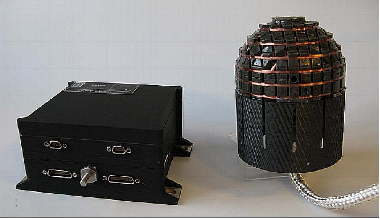
VFM instrument: The VFM (fluxgate type) is based on the fluxgate transducer using a ringcore with amorphous magnetic material, which has a very low noise (10-20 pT rms). It has an extremely high stability < 0.05 nT/year. VFM consists of a CSC (Compact Spherical Coil) sensor, non redundant, mounted on the deployable boom, an internally redundant data processing unit (DPU) and the connecting harness. The spherical coils that create a homogeneous vector field inside the sphere are mounted on an isotropic and extremely stable mechanical support. In feedback conditions the sensor is used as a nulling device and the coils define uniquely the magnetic axes of the sensor. The VFM exhibits high linearity (< 1ppm), a component accuracy of 0.5 nT and precision of 50 pT rms.
The operation of the fluxgate sensor is based on the extreme symmetry of the positive and negative magnetic saturation levels of the ferromagnetic sensor core material. Continuous probing of the core saturation levels by a high frequency excitation magnetization current enables the sensor to detect deviations from the zero field with only tens of pT noise and sub-nT long term stability.
The mounting of the VFM sensor is using a sliced adaptor ring. The optical bench ensures mechanical stability of the system. Three star trackers provide full accuracy attitude.
Instrument mass, power consumption | 1 kg, 1 W |
Dimension of sensor head (CSC) | 82 mm Ø |
Dimension of DPU | 100 x 100 x 60 mm |
Data rate |
|
Dynamic range | ±65536.0 nT to 0.0625nT (21 bit) |
Omnidirectional linearity | ±0.0001% of full scale (±0.1nT in ±65536nT) |
Intrinsic sensor noise | 15 pTRMS in the band 0.01-10 Hz (6.6 pTRMS Hz-1/2 at 1 Hz) |
Intrinsic electronics noise | 50 pTRMS in the band 0.01-10 Hz (15 pTRMS Hz-1/2 at 1 Hz) |
Sampling rate | 50 Hz, linear phase filter, -3dB frequency 13.1 Hz |
Temperature range | -20ºC to +40ºC (Operating performance) |
Thermal behavior |
|
Zero stability (thermal & long term) | < ± 0.5 nT |
Absolute accuracy of Ørsted magnetometer parameters (relative to ASM & STR): | |
- Offset | < 0.2 nT (~120 dB) |
- Scale factors | < 0.0005% |
- Axes orthogonality | < 0.0006º (~2 arcsec) |
- Axis alignment | < 0.0002º (~7 arcsec) |
Ørsted magnetometer with 3 offsets, 3 scale factors & 3 angles for 6.5year: | |
Accuracy | < 0.5 nT |
The µASC (micro Advanced Stellar Compass) of DTU Space provides the high accuracy, inertial attitude determination for the Swarm vector magnetometer. The microASC is a fully autonomous, internally hot/cold redundant star tracker, featuring up to four cameras. The microASC features a split DPU (Data Processing Unit) and CHU (Camera Head Unit) enabling the low power dissipation and very low magnetic disturbance CHU, to be placed close to many types of science instruments, including the CSC sensor (see µASC description below).
Inter-calibration: determining the internal angels between the CSC and the three CHUs: The optical bench provides a mechanically stable platform for the CSC and the three CHUs and will ideally fixate the internal angles between these. The prime objective of the inter-calibration is to establish the internal angles with the highest possible accuracy. The measurement frame of the CSC sensor is defined by the orientation of the compensation coils on the outside of the CSC sensor sphere. These coils form a nearly orthogonal triad, which has been thoroughly calibrated and orthogonalized prior to the mounting on the bench structure. Similarly the measurement frame of any of the CHUs is defined by the mechanical arrangement of the optics relative to the CCD sensor of the unit. Also this measurement frame has been established prior mounting the unit on the bench.
Despite the effort to minimize thermo-elastic deformations and the effort to make the platform as stiff and stable as possible, small residual variations exists. A secondary objective for the inter-calibration is therefore to assess the size of these residual errors, e.g. gravity release effects.
Finally, the mounting of the sensor units to the stiff optical bench will cause stresses to be built into the mounting interfaces. These stresses may cause minute changes to the internal calibration of the sensors. A third objective of the inter-calibration is therefore to verify the pre mounting calibration of the sensor units.
ASM (Absolute Scalar Magnetometer)
ASM is provided by CNES (French Space Agency) and CEA-LETI (French Atomic Energy Commission - Laboratoire d'Electronique de Technologie et d'Instrumentation), Grenoble, France. The objective is to measure magnetic field strength and to calibrate the VFM device to maintain the absolute accuracy during the multi-year mission. ASM is positioned at the very tip of the boom. The required main performance characteristics of the ASM are: absolute accuracy of < 0.3 nT (2σ), resolution < 0.1 nT within its full-scale range of 15000-65000 nT. 137) 138) 139) 140) 141) 142) 143) 144) 145)
Measurement concept: To overcome the limitations of the OVM (Overhauser Magnetometers) identified during the Oersted and Champ programs, a new magnetometer has been designed for the Swarm mission. The ASM pumped helium magnetometer relies on a low pressure helium vapor as the sensing medium (Figure 75), with the optical pumping process the counterpart of the dynamic nuclear polarization. 146) 147)
One important difference is however due to the fact that the optical pumping is a much more efficient polarization method, leading to an almost complete polarization. As a consequence, the signal amplitude does no longer depend on the magnetic field strength and a resolution of 1 pT/ (Hz)1/2 is now obtained over the complete measurement range.
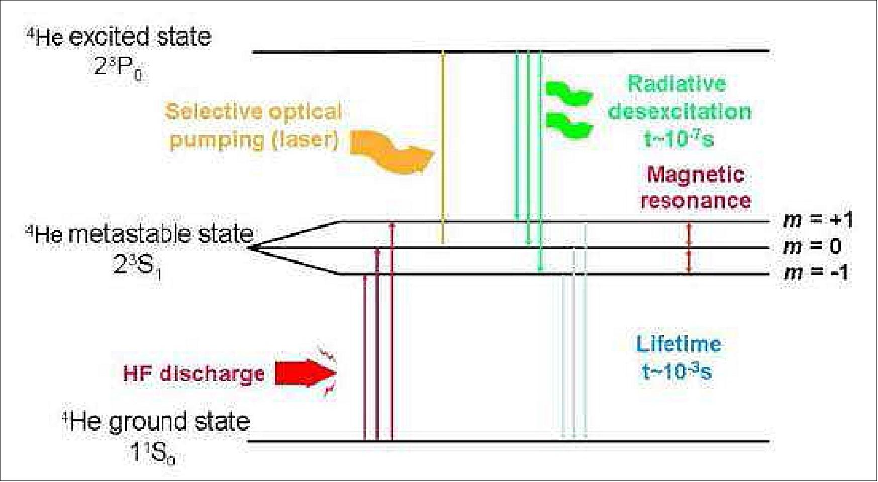
As compared to most optically pumped magnetometers, the ASM operates with linearly polarized pumping light instead of circularly polarized light. The main reasons for that choice are the following:
- the strong interaction between the laser pumping beam and the helium atoms can in general affect their energy level and result in so-called light shifts whenever the pumping light wavelength is detuned from the helium transition center wavelength. Now using linearly polarized light suppresses this effect, thus significantly increasing the instrument’s accuracy.
- the key parameter governing the optical pumping angular dependence is then the direction of the laser polarization, whereas it is the propagation direction of the pumping beam that matters in circularly polarized light. Now when trying to design an isotropic instrument, i.e an instrument whose performances are independent of the sensor attitude, it is obviously easier to control the direction of the linear polarization than to rotate the whole sensor in order to align it properly with respect to the magnetic field direction. In our case the isotropy is thus simply achieved thanks to the use of an amagnetic piezoelectric motor which permanently controls the laser polarization and the RF magnetic field directions so that they are both perpendicular to the static magnetic field. The resulting magnetometer architecture is illustrated in Figure 76.
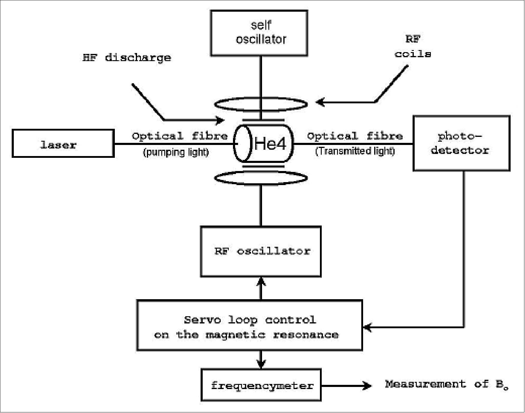
Contrary to the Overhauser solution based on a design trade-off between instrument’s resolution and omnidirectionality, the helium magnetometer is always operated in the optimal operational conditions thanks to this servo loop, but this is achieved at the expense of the use of a dedicated mechanism. As for the sensor anisotropy, resulting from a combination of induced and remanent contributions, a typical signature corresponding to the flight configuration is presented in Figure 77.
As for the environment susceptibility, the ASM significantly broader resonance line (close to 70 nT as compared to less than 7 nT for the OVM) reduces the impact of inhomogeneous magnetic fields on the magnetometer performances, while the principles of operation and architecture of the helium device makes it robust to low frequency radiated magnetic fields, thus making the EMC specifications much easier to meet in that respect.
Last but not least, the short metastable helium relaxation time (of the order of one millisecond) results in a much higher bandwidth for the helium magnetometer than was the case for the NMR sensors. While this feature is of no direct interest for the calibration of the vector instruments (the scalar data are sampled for that purpose at a fixed 1 Hz frequency), it opens new opportunities for the exploitation of the scalar instrument.
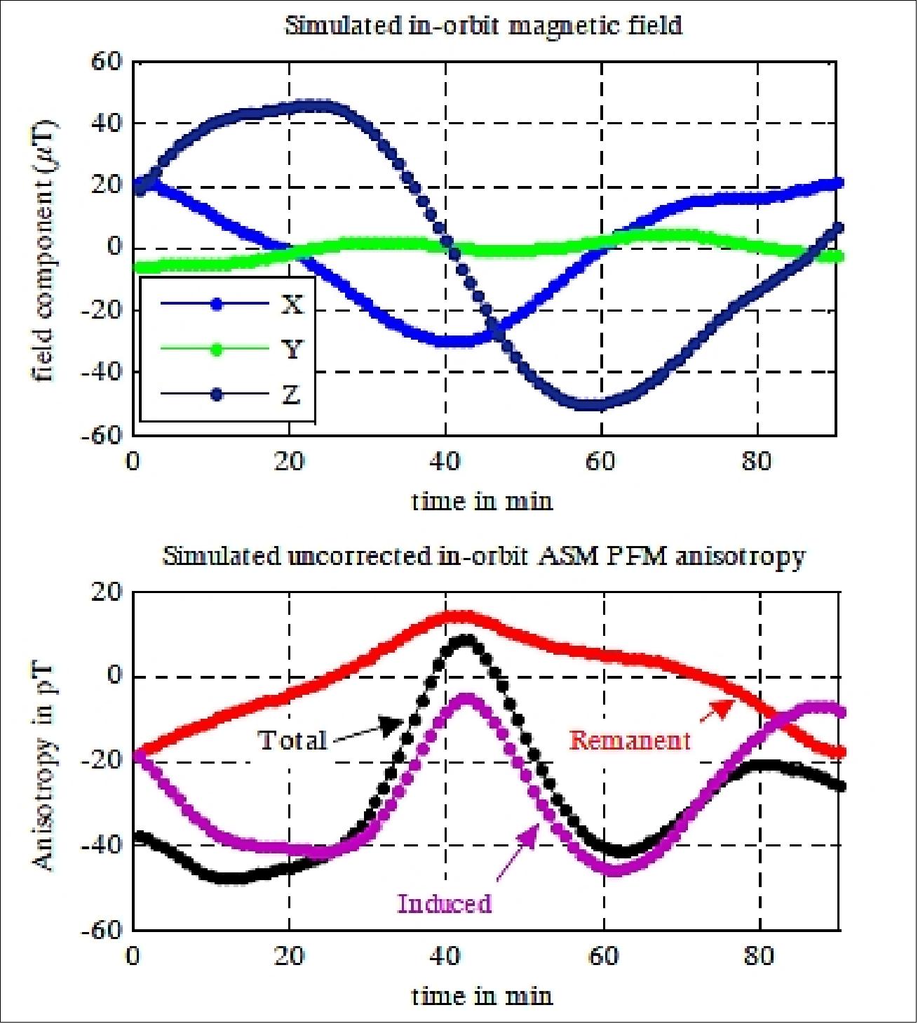
Instrument: The ASM magnetometer is based on the ESR (Electron Spin Resonance) principle and makes use of the Zeeman effect which splits the emission and absorption lines of atoms in an ambient magnetic field. The pattern and amount of splitting is a signature of the magnetic field strength. The optically pumped helium magnetometer uses a High Frequency (HF) discharge within a gas cell to excite 4He atoms from the ground state to the metastable state. This metastable level is split by the Earth magnetic field into 3 Zeeman sublevels. The separation of those sublevels is directly proportional to the ambient field strength and equals half the gyro frequency (eB/2m - where m is the electron mass).
Given the role of the laser in the ASM instrument, the following specifications have to be met:
• Wavelength stability with piezoelectric modulation piezoelectric modulation around the D0 transition : λ=1082.908 nm in air standard (std)
• RIN (Relative Intensity Noise) lower than -135 dB (Hz)1/2 at 1 kHz and 2 mW of output optical power
• Spectral linewidth lower than the D0 absorption width of 1.7 GHz
• Specific space environment and space design requirements.
The fiber laser consists of a pump laser diode, a WDM (Wavelength Division Multiplexer), an Yb doped FBG (Fiber Bragg Grating), an optical isolator and a splitter to allow a feedback control. In this architecture, the noise reduction loop acts on the pump diode current by detecting the low frequency fluctuations of the output optical power from the dedicated photodiode located in the 20 % splitter output. The corresponding block diagram is presented in Figure 78.
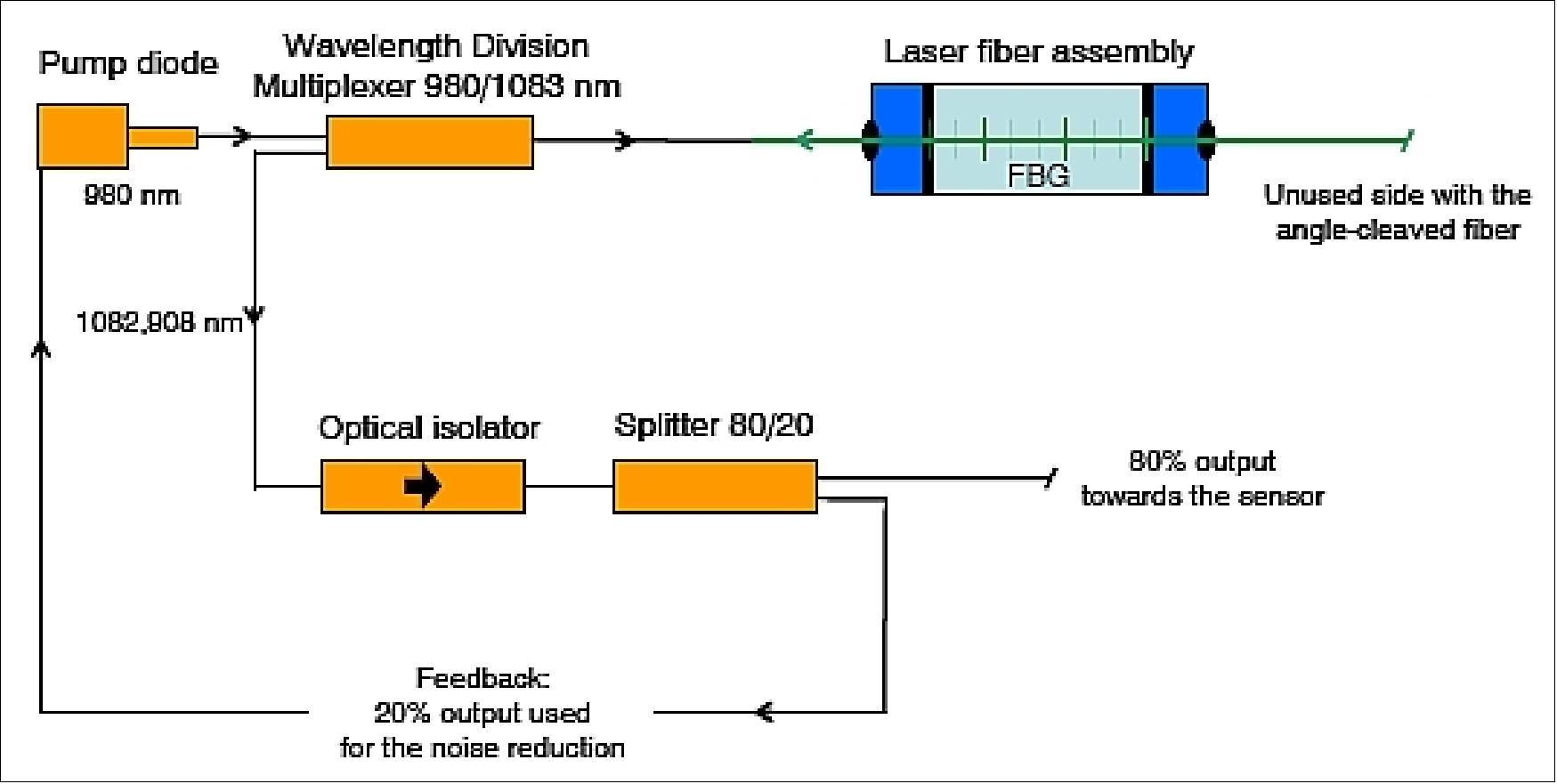
Athermal design of the LFA (Laser Fiber Assembly): The ASM laser has to be able to pump the 4He at 1082.908 nm (in air std) within the temperature range of [-5ºC; +50ºC] which is the specified qualification operating temperature range of the ASM electronics on the Swarm satellites. One of the main challenges to take up for the LFA conception was to reduce the thermal wavelength drift as much as possible in a passive way. We could have used, for example, a 1083 nm laser diode with a thermo-electric Peltier device but the laser consumption would have been highly increased.
The role of the piezoelectric actuator (made by the CEDRAT Group) is to modulate and to allow a fine tuning of the laser wavelength around the 4He D0 transition. A picture of the final LFA design is given in Figure 79.
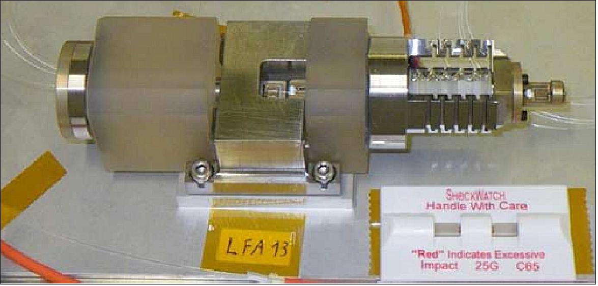
Legend to Figure 79: The pre-stressed piezoelectric actuator on the right is glued on the Zerodur®; the LFA is then fixed in the ASM electronics box with the titanium bridge put upon the Zerodur®.
Another challenge to take up was the design of a suitable fixation system of the LFA allowing it to comply with the shocks and vibrations specifications. A solution has been developed using a titanium bridge, coned-disc springs (also known as Belleville washers) and elastomers (with suitable thickness and hardness, and a low outgassing characteristic). - The pieces of elastomer are located under the LFA and between the titanium bridge and the LFA in order to dampen any tri-axis vibrations or shocks. This fixation system has successfully passed the vibrations and shocks qualification tests. The final titanium fixation bridge is shown on the LFA of Figure 79.
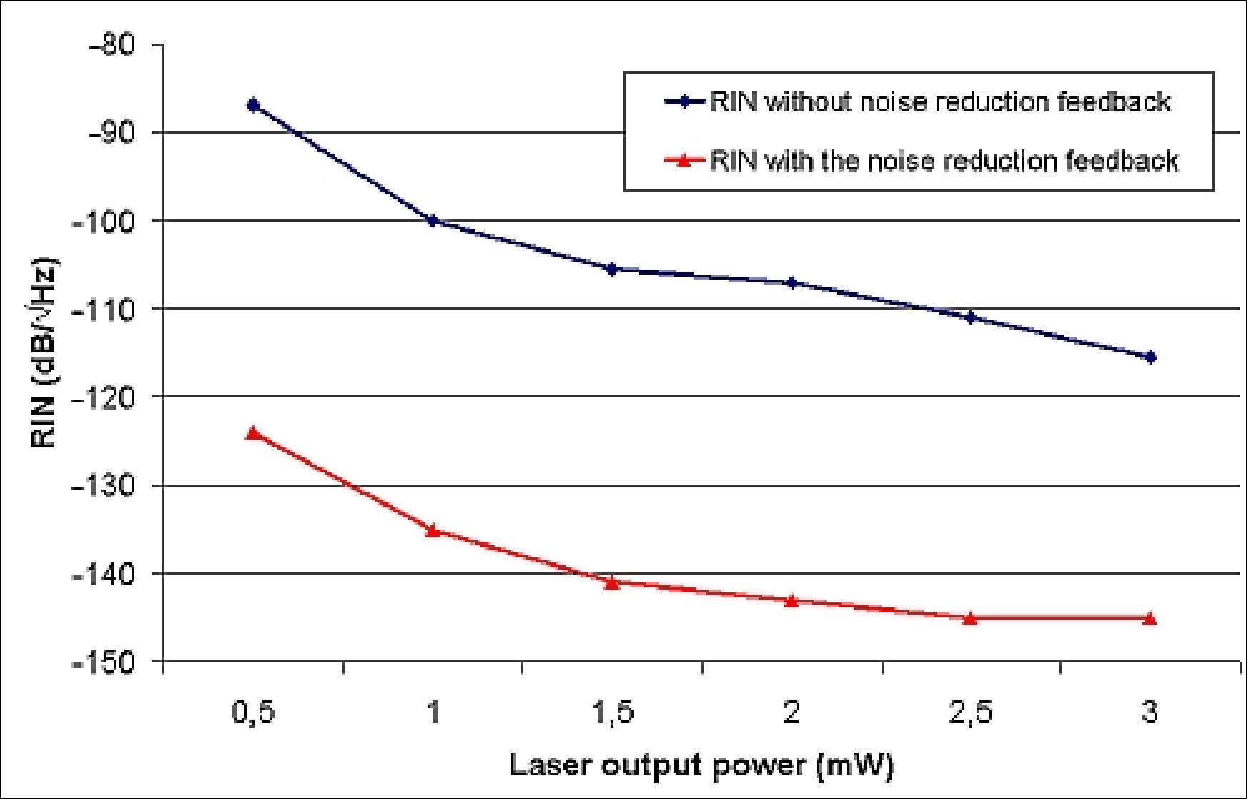
RIN performance: For both consumption and simplicity reasons, in the ASM instrument it has been chosen to detect the magnetic resonance signals coming from the 4He cell around 1 kHz, which corresponds to the 1 kHz modulation of the continuous part of the LA0 magnetic resonance signals between the Zeeman sub-levels. This signal is high enough to allow the measurement of the magnetic field with a low noise laser: the corresponding RIN measurement of the ASM laser is shown in Figure 80 (obtained from an electronic spectrum analyzer and an InGaAs photodiode). As shown, the low frequency feedback control loop presents the opportunity to reduce the RIN from about -105 dB (Hz)1/2 at 2 mW of output power around 1 kHz down to -140 dB (Hz)1/2. The low noise laser specifications are thus met.
Instrument mass, power consumption | 3 kg, 5.3 W |
Size of sensor head | 40 mm x 60 mm |
Size of DPU | 200 mm x 150 mm x 100 mm |
Dat rate | 0.35 MByte/ day |
Dynamic range | 15000 - 65000 nT full scale |
Absolute accuracy | < 0.3 nT (2σ) |
Omni-directional response | < 0.1 nT angular dependence |
The instrument assembly consists of a DPU (Digital Processing Unit) and a separately installed sensor connected to the electronic box by a bundle of optical fibers and electrical cables (harness). A specific sensor bracket is designed to mechanically interface 2 identical sensors with the satellite boom (a cold redundancy has been chosen for Swarm, each sensor being connected to a dedicated DPU located within the satellite main body).
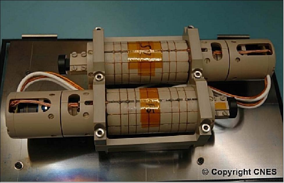
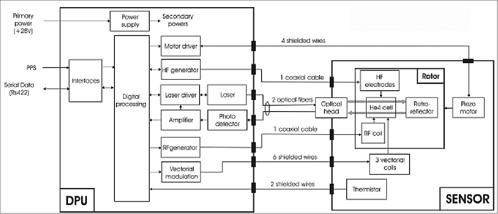
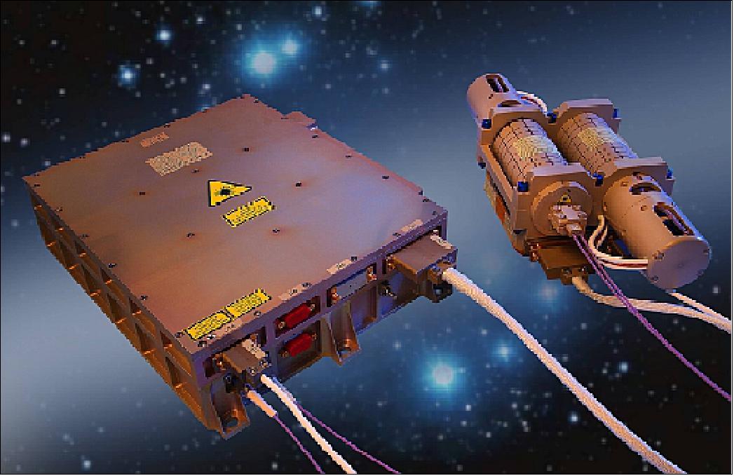
The ASM characteristics make the instrument ideally suited not only for the traditional role of scalar magnetometers as absolute references for the calibration of the on-board vector instruments, but also for extended operational capacities, such as higher frequency scalar measurements (of potential interest for magnetosphere studies for the low frequency part of the spectrum) or autonomous scalar / vector operations. Last but not least, the helium magnetometer can be operated in a zero field configuration with only very minor evolutions in the sensor overall design, thus extending its initial capabilities to new missions in planetary exploration (Ref. 146).
Electromagnetic cleanliness: Differential scalar measurements have been performed throughout the ASM development phases up to the satellite final ground magnetic tests. This allowed first to select the sensors parts in order to minimize their residual magnetic signature and second to evaluate the accuracy of the magnetic data that will be delivered by the ASMs for the three satellites of the Swarm constellation both at instrument and satellite level. This differential method has been adapted to the various rather challenging tests configurations met within the Swarm program. It allowed to demonstrate that the ASM performances meet the mission requirements, with measurement uncertainties below 25 pT. It finally contributed to improve the quality of the magnetic measurements that were carried out at satellite level and check the perturbation models that had been established. 148)
Characterization and removal of thermomagnetic perturbations onto ASM instrument. 149)
A step-by-step perturbation identification and removal process has then been set up in order to characterize the global perturbation and has resulted in several hardware upgrades. Thanks to dedicated scalar differential measurements performed in the CEA-Leti Magnetic Characterization Facility of Herbeys, all elements which have been characterized as sources of thermomagnetic perturbations have been progressively removed or replaced.
The test process has led to several hardware upgrades (3 in total) of both the mechanical interface of the ASM with the satellite boom and later even some ASM components. The original titanium interface bracket including the heaters for the ASM thermal control has been replaced by CFRP (Carbon Fiber Reinforced Polymer) components and the ASM internal harness connectors have been removed. These successive evolutions can be simply summarized as follows: the less metallic material submitted to thermal gradient in the vicinity of the ASM, the smaller
the perturbation, which makes perfectly sense with thermomagnetic generated effects.
In the end, this exhaustive test campaign has demonstrated the very efficient reduction of thermomagnetic perturbations generated in the close environment of the ASM: the remaining maximum effects have been characterized in the 20-30 pT +/- 5 pT peak-to-peak range (Figure 4) which is well below the accuracy specification of 300 pT (2σ) allowed for ASM for the Swarm mission
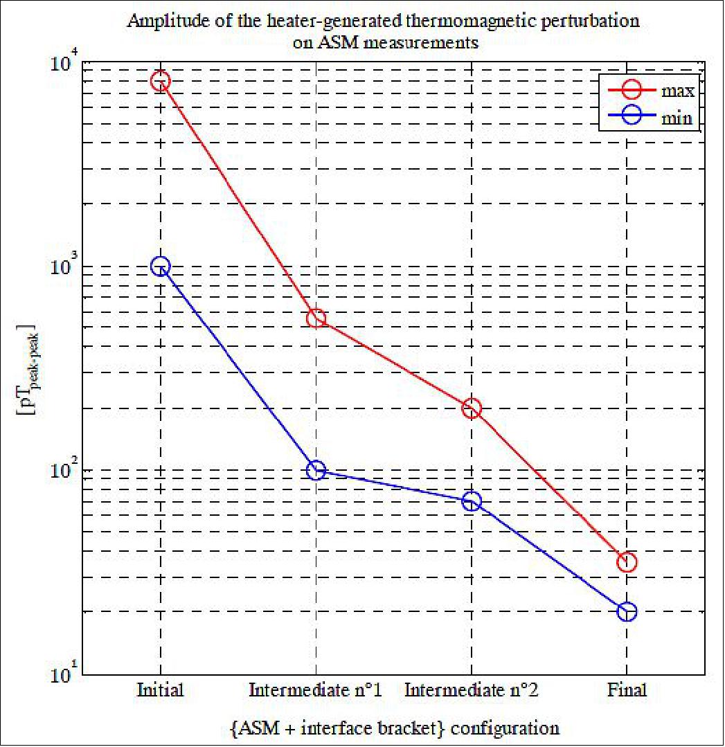
Thanks to the removal and/or replacement of metallic components in the close environment of the ASM sensor, it has been possible to get rid of these perturbations before the launch of the Swarm satellites. The study puts further emphasis on one of the basic design rules for the conception and integration of magnetic sensors on-board space vehicles: avoid as much as possible metallic elements in the vicinity of these instruments, even if they do not show any static magnetic signature. They can still give rise to magnetic perturbations if they are submitted to thermal gradients, which turn to be very difficult to compensate for by modelling as these elements are never simple in shape and as it also requires a very precise 3D knowledge of their internal temperature distribution.
EFI (Electrical Field Instrument)
EFI, also referred to as CEFI (Canadian Electric Field Instrument), is provided by Canada (CSA funding, design by the University of Calgary, with ComDev Ltd. of Cambridge, Ontario as instrument manufacturer). The CEFI sensor is based on SII (Suprathermal Ion Imager)-a Canadian particle detector design that has already proven its capability - to gather precise measurements of ion winds. The goal of the CEFI instrument is to characterize the electric field about the Earth by measuring the plasma density, drift, and acceleration at high resolution; also for plasma density mapping in conjunction with GPS.. CEFI derives its heritage from the CPA (Cold Plasma Analyzer) instrument on Freja, the Nozomi TPA instrument and the CUSP, JOULE and GEODESIC sounding rocket missions. 150) 151) 152) 153) 154)
The plasma ion measurements are derived from energy-angle distributions that are generated by two orthogonal 2D electrostatic analyzers on each satellite. The ion bulk flow velocity and temperature are related to the distribution moments by transfer functions whose form are determined from simulations of the analyzers. The electric field is determined from measurements of the ion velocity and the magnetic field. 155)
The main sources of error come from uncertainties in the instrument transfer functions, the sensor-to-plasma potential difference, particle Poission noise, galactic cosmic ray event, and detector gain variations.
The CEFI instrument is comprised of three main parts: the SII (Suprathermal Ion ImagerI) sensors, the LP (Langmuir Probe) sensors, and the Electronics Assembly. The electronics assembly contains all of the electronics necessary to support power supply, sensor data acquisition, instrument control and communications with the spacecraft bus. The electronics assembly and SII sensors will be positioned on the ram face of each Swarm spacecraft along with the Langmuir probes positioned preferably on the ram and nadir faces of each spacecraft and connected to the electronics assembly with wire harnesses.
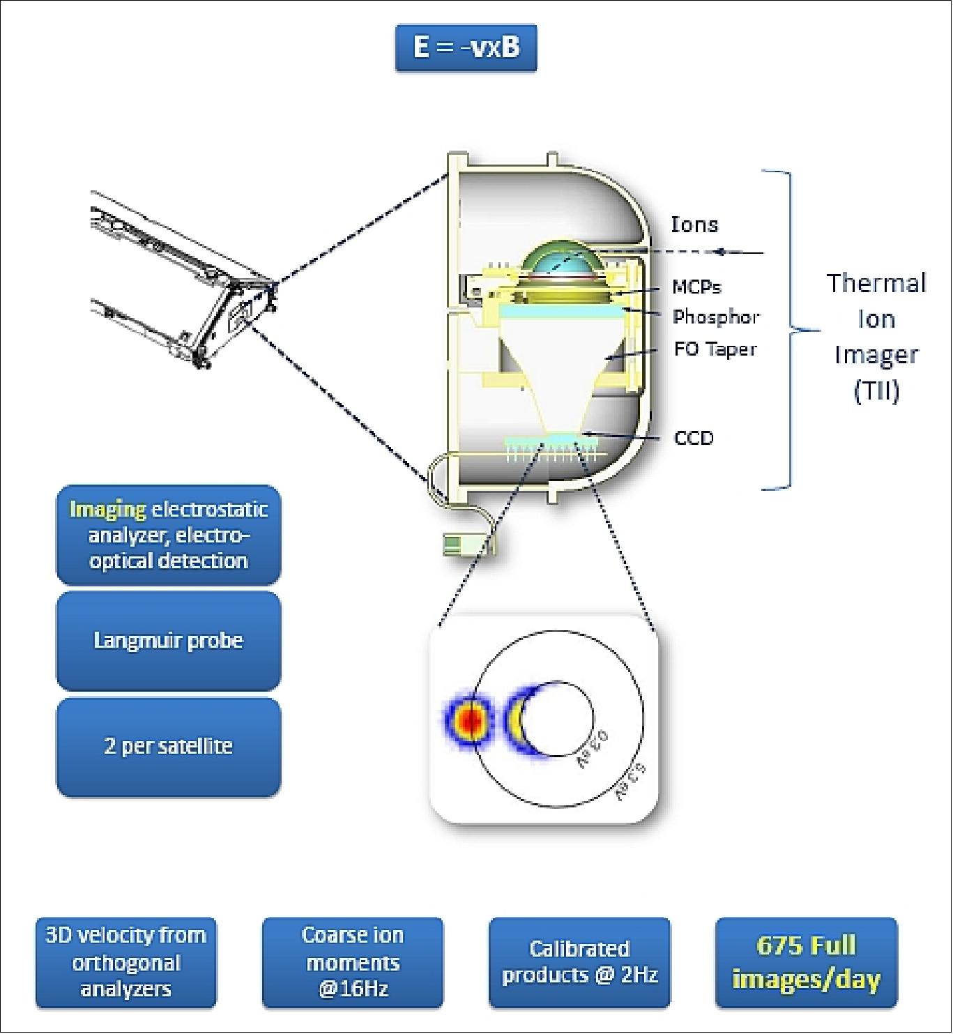
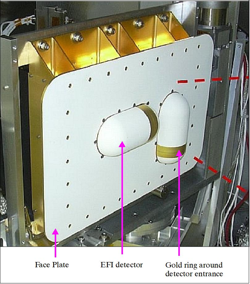
The SII sensors are of CPA heritage; they are using a unique particle focusing scheme developed at the University of Calgary. Ions enter a narrow aperture slit and are then deflected by a pair of hemispherical grids that create a region having electric fields directed radially inward. Incoming low-energy positive ions are accelerated toward the center of the spherical system, whereas ions with larger kinetic energies travel farther toward the edge of the detector, creating an energy spectrum as a function of detector radius (Figure 87).
Particles arriving from out of the plane of Figure 87 land at different azimuths on the image plane. The resulting image from each SII sensor is a 2D cut through the ion distribution function, from which one can calculate ion density, drift velocity (2D), temperature, and higher-order moments. The two SII sensor head assemblies are oriented such that the aperture slits are oriented perpendicularly to each other, enabling 3D characterization of the ion distribution.
Range of operational conditions:
• Natural variability
- Ion densities (108-10 m-3)
- Ion and electron temperatures (0.1-0.5eV)
- Ionospheric plasma flow (~200 m/s)
• Active biasing of face plate
• Passive biasing of material components associated with different work functions and contact potentials.
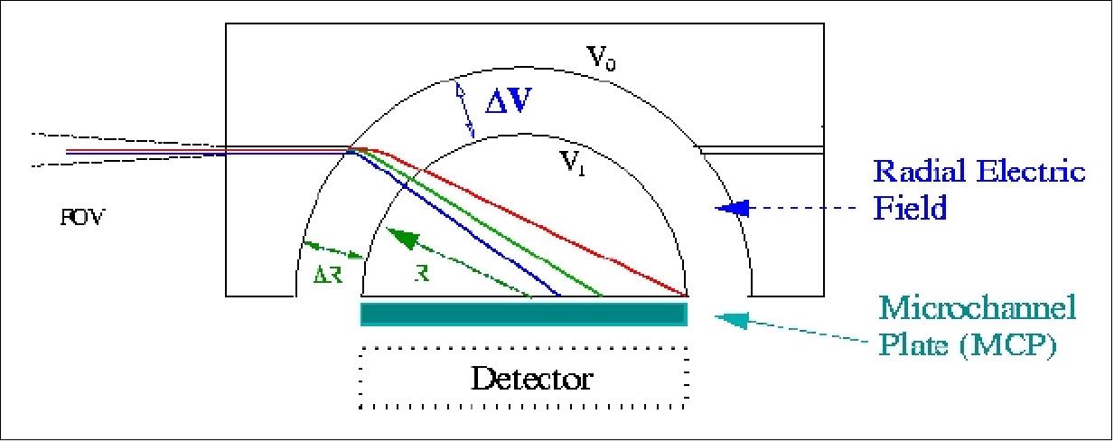
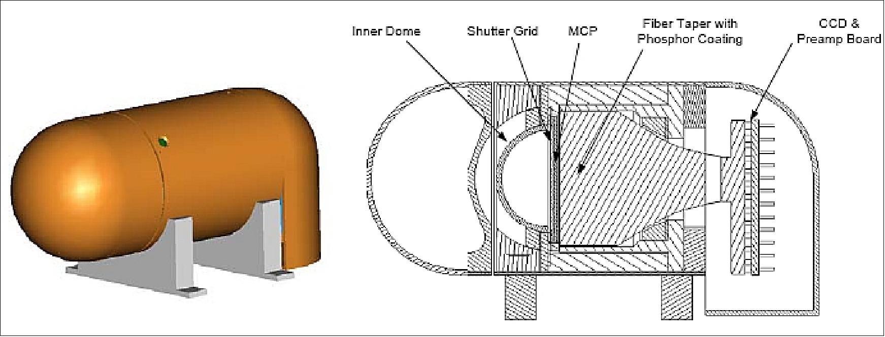
When the charged particles strike the MCP Microchannel Plate) detector, the signal is amplified through secondary emission processes. The voltage applied across the MCP controls the gain of the device. In parts of the orbit where ion flux is high, the voltage applied to the front surface is reduced to limit the gain of the device and preserve its life. This gain adjustment is part of an automatic gain control realized through the use of a feedback loop using the CEFI instrument faceplate current as a control input. Where sufficient gain control cannot be achieved via the MCP voltage alone, an electrostatic shutter will gate the incoming ions with duty cycles ranging from 100% to well below 1%.
A Langmuir Probe assembly is part of the CEFI device to provide measurement of electron density, electron temperature and spacecraft potential. The LP design is based on hardware flown on the Cluster and Rosetta missions of ESA and was developed by the Swedish Institute of Space Physics. The overall height of the LP sensor is 10 mm.
The instrument electronics assembly includes the following electrical subsystems:
• Instrument controller
• Detector readout electronics
• HVPS (High Voltage Power Supply)
• LVPS (Low Voltage Power Supply). The primary function of the LVPS is to generate low voltages for other electronics within the Swarm CEFI instrument.
• Langmuir probe assemblies.
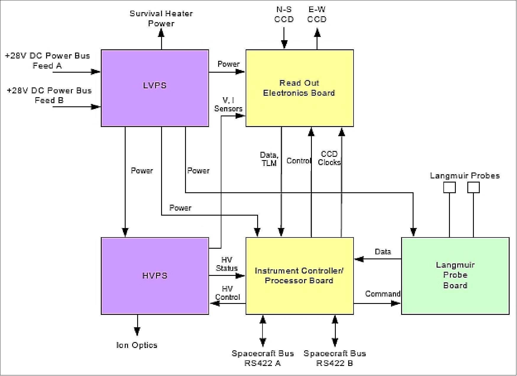
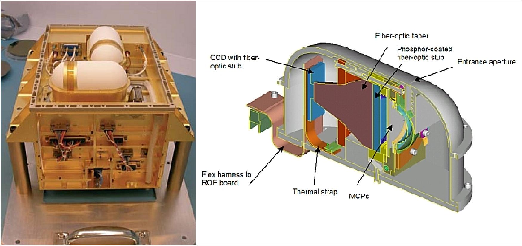
MAC-04 (Micro Accelerometer-04)
MAC-04, or simply ACC, is an electrostatic accelerometer instrument assembly designed and developed at VZLU (Výzkumný a zkušební letecký ústav, a.s. - Aeronautical Research and Test Institute), Prague, Czech Republic. EADS Astrium (as prime contractor to ESA for the Swarm mission) awarded the MAC-04 contract to VZLU in March 2008. VZLU is the lead of a MAC-04 consortium, involving 14 Czech institutions and companies. 156)
The overall objective is to measure non-gravitational perturbing accelerations (time and spatial variability), such as air drag, winds, Earth albedo (reflected solar radiation from the cloud/snow coverage and the thermal radiation of the Earth), and solar radiation pressure on the spacecraft. In-situ air density measurements together with magnetic data can be used to obtain new insights on the geomagnetic forcing of the upper atmosphere.
Typical magnitudes of non-gravitational forces are presented in Table 7. For spacecraft altitudes below 800 km the atmospheric drag is the dominant acceleration; at higher altitudes, the direct solar radiation pressure and other radiative forces are increasing in dominance.
Acceleration origin | Acceleration magnitude (ms-2) |
Atmospheric drag | 10-4 to 10-9 |
DSRP (Differential Solar Radiation Pressure) | 2.9 x 10⁻⁸ |
Albedo | 10-8 to 10-9 |
Reflected infrared radiation | 4 x 10⁻⁹ |
All these radiation effects have a common feature – namely a slow change of magnitude with time and position in orbit. However, for the solar radiative effects, the illumination of the spacecraft is a precondition for any acceleration detection in its orbital path.
The solar activity has a direct impact on atmospheric drag. The thermosphere usually expands and contracts in line with the sun's 11 year solar cycle. During solar maximum when solar activity increases, it causes the thermosphere to heat up — reaching temperatures of 1100ºC — and expand. The opposite happens during solar minimum. As solar activity increases, EUV (Extreme Ultraviolet) radiation heats our planet's gaseous envelope, causing it to swell and reach farther into space than normal. However, despite of the sun's possible rapid fluctuations, Earth's thermosphere response is a fairly slow process. These considerations led to the design performances of the MAC-04 accelerometer as shown in Table 8.
Linear acceleration range | ± 10-4 m s-2 |
Angular acceleration range | ± 3 x 10⁻⁸ rad s-2 |
Measurement bandwidth range | 10-4 to 10-1 Hz |
Resolution for linear acceleration better than | 10-9 m s-2 |
Resolution for angular acceleration better than | 10-7 rad s-2 |
Overall random error better than | 5 x 10⁻¹⁰ m s-2 |
The accuracy of a component of the linear acceleration vector shall be better than 0.2% of the measured value | |
Measurement Principle
The MAC-04 assembly is composed of a cubic proof mass which is free-floating in the cubic cavity. The center of the sensor will be accommodated in the spacecraft’s center of gravity. The proof mass is separated from external influences by the satellite structure and the construction of the micro-accelerometer.
Free motion of the proof mass is realized by virtue of the gravitational law. The cavity is rigidly connected to the satellite body. The gravitational as well as all perturbing forces acting on a satellite produce their acceleration contributions which are identical to the one of cavity. The difference between the acceleration of the cavity and the acceleration of the proof mass is the sum of all accelerations produced by the non-gravitational forces acting on a satellite.
A precise measurement of the proof mass position enables to properly detect its small relative displacements with respect to the satellite-fixed cavity. Applying a known electrostatic force, the instrument can compensate and measure the action of the non-gravitational forces. This proof mass position control is performed by a feedback loop of the servo control electronics.
A block diagram of the sensor control circuit is shown in Figure 129. Part of the block diagram placed in the dashed border represents the dynamics of the proof mass. The constants A1, A2 and A3 represent the shape and geometry of the electrodes and their distance to the proof mass.
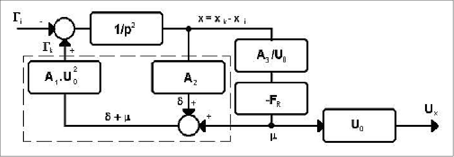
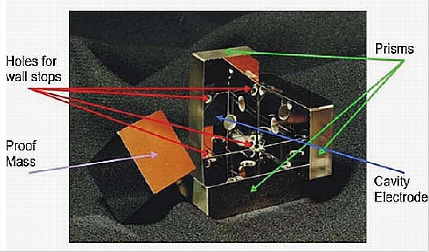
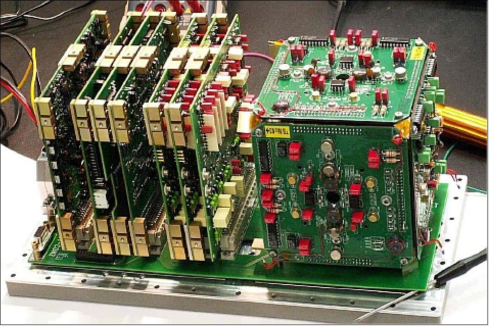
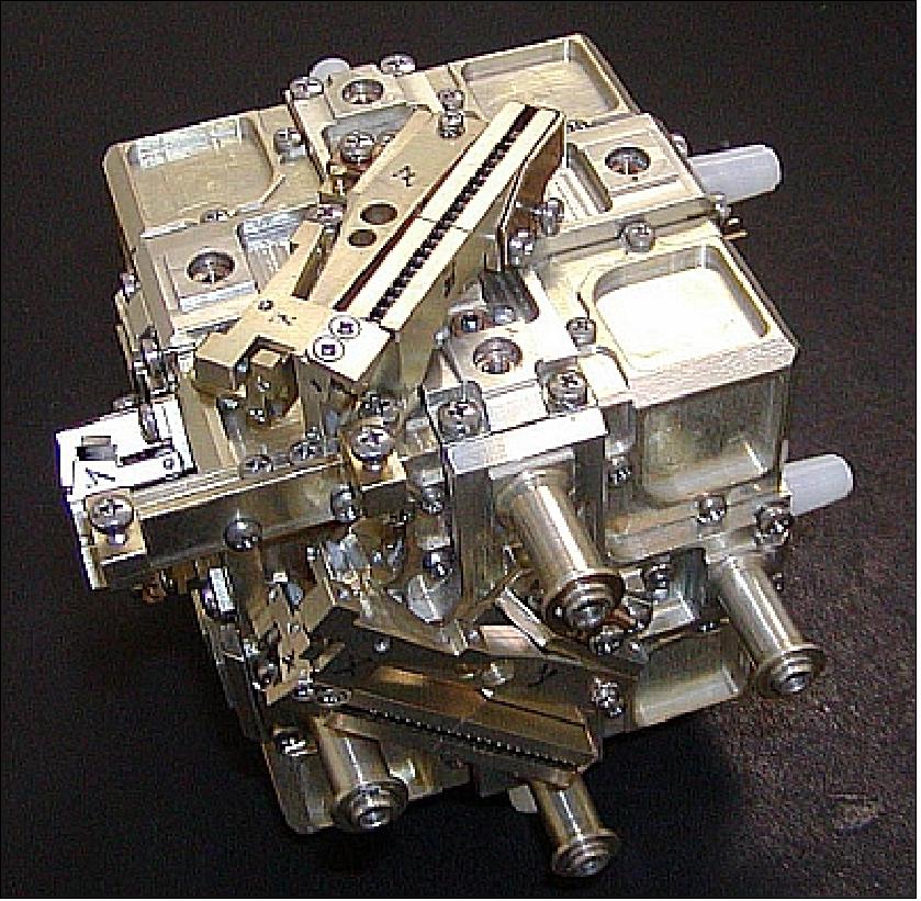
MAC-04 science data output 1Hz rate:
- Linear acceleration: 3 vector components
- Angular acceleration: 3 vector components
- Linear positions: 3 vector components
- Angular positions: 3 vector components
- Temperatures: 8 sensor values.
Some Background of Czech Accelerometer Instrument Projects in Spaceflight
During the last two decades, the Czech Republic has developed several accelerometer instrument models within the framework of the non-gravitational accelerometer program. There is great interest among the theoreticians in satellite dynamics since our understanding of the non-gravitational effects is rather limited. In many cases, only rough phenomenological models are available. In situ measurements of the non-gravitational effects have thus great importance for checking the theoretical concepts. The MAC (Micro Accelerometer) program (formerly referred to as MACEK) is devoted to such measurements with an expected threshold up to 5 x 10-11 ms-2 .
Table 9 provides an overview of the various spaceborne missions whose payload included a MAC instrument. The obtained measurements are of different quality. The first two instrument models (flown on Resurs-F1 and on the STS-79 flight of the Space Shuttle) were mainly of in-flight technology verification nature. The MIMOSA project was the first small satellite dedicated to the research of the thermosphere. Unfortunately the failure of unlocking in one axis spoiled the mission goal.
The first MAC-04 instrument of VZLU, developed under in the frame of the project TEASER (Technological Experiment And Space Environment Resistance), was launched with the Russian Tatiana-2 mission in Sept. 2009. The project was funded Ministry of Industry and Trade of the Czech Republic. - However, after spacecraft separation from the upper stage of the launch vehicle, the satellite stabilization system did not work correctly (infrared Earth sensor failed). When all trouble shooting didn't bring any tangible results, the communication with the spacecraft was terminated after one month of “operations” with the spacecraft.
As of mid-2010, the development of the MAC-04 instrument for the Swarm mission is completed and instrument qualification for the mission is underway. Although the measurement principle is quite simple, past experiments showed high demands on the precise adjustment of the accelerometer in ground conditions. Moreover the complexity and the high precision adjustment of the sensor mechanical parts in combination with electronics properties (e.g. temperature dependence) represent a challenging task in the MAC-04 accelerometer verification.
Launch of mission, Instrument model ⇒ | MAC-01 | MAC-02 | MAC-03 | MAC-04 |
June 23, 1992 | Resurs-F1 (proof of concept flight) |
|
|
|
Sept. 16-26, 1996 |
| STS-79 |
|
|
June 30, 2003 |
|
| MIMOSA |
|
Sept. 17, 2009 |
|
|
| Tatiana-2 |
2012 |
|
|
| Swarm |
Instrument model ⇒ | MAC-01 | MAC-03 | MAC-04 |
Linear range (ms-2) | ±4 x 10⁻⁴ | ±5 x 10⁻⁵ | ±2 x 10⁻⁴ |
Angular range (rad s-2) | ±9 x 10⁻³ | ±9 x 10⁻³ | ± 9 x 10⁻³ |
Resolution for linear acceleration (ms-2) | 3 x 10⁻¹⁰ | 2 x 10⁻¹⁰ | 2 x 10⁻¹⁰ |
Temperature resolution (ms-2 K-1) | 10-7 | 3 x 10⁻⁹ | 3 x 10⁻⁹ |
Stability (ms-2 day-1) | - | 10-8 | 10-8 |
The Czech Republic formally became ESA's 18th Member State on 12 November 2008. Already in 1996, Czech Republic signed the formal Framework Cooperation Agreement. In November 2003, however, the Czech Republic became an ESA European Cooperating State by signing the Plan for European Cooperating States Agreement (PECS Agreement) and entering the ESA PECS Program. 157)
LRR (Laser Retro Reflector)
The LRR instrument is being provided by GFZ Potsdam. The objective is spacecraft POD (Precise Orbit Determination) to cm-level accuracy by SLR (Satellite Laser Ranging).
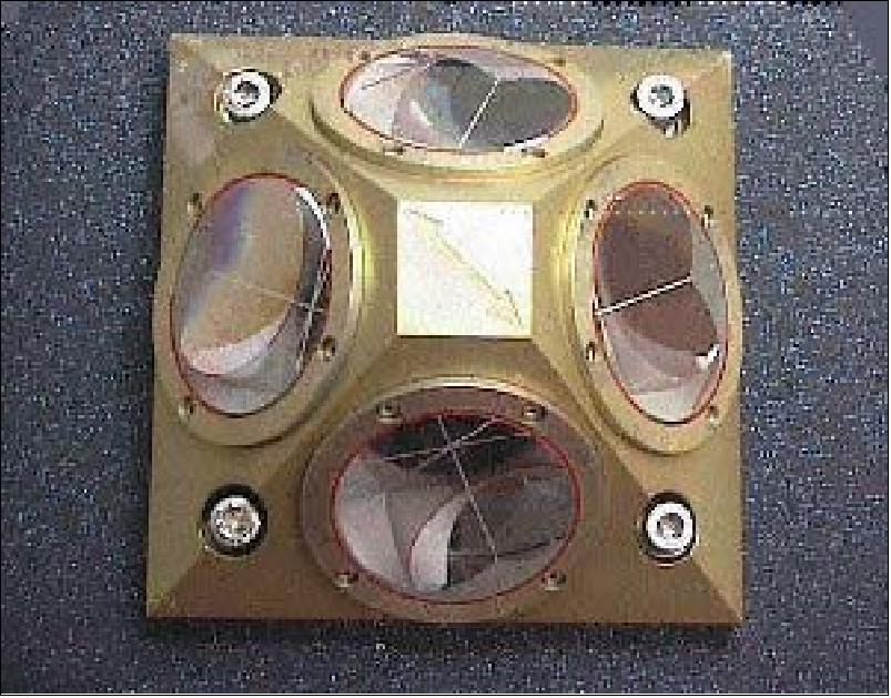
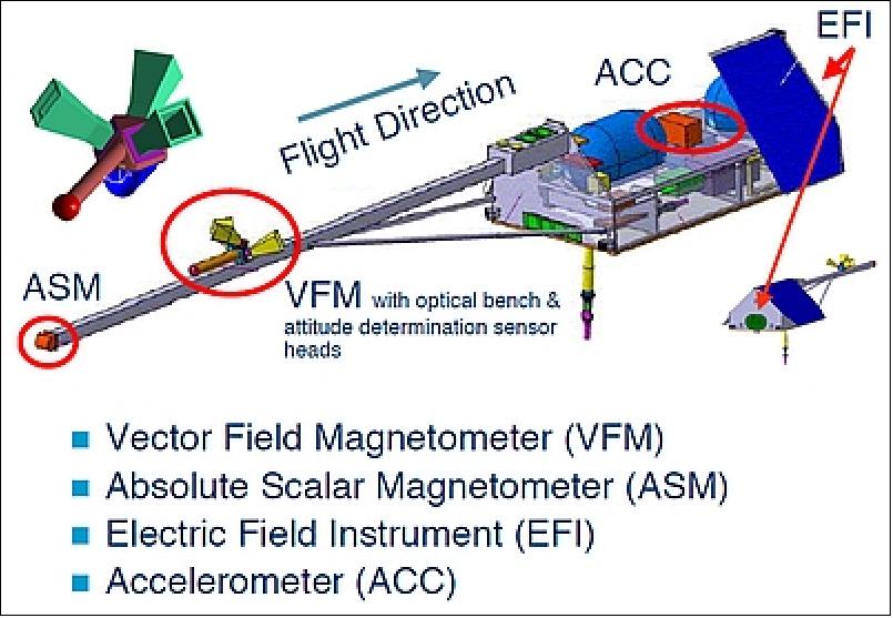
Internal Field Components | |||||
Research objective | Time range | Spatial range | Signal range | Signal at certain wavelength (wl) | Measurement |
Core dynamics and geodynamo processes | static | 300 km to global | < 65000 nT | 2.35 nT @ 3000 km wl | B-field vector, attitude & position |
3 months to decades | 2500 km to global | ±200 nT/year | 0.025 nT/3 months @ 2850 km wl | ||
Lithospheric magnetization | decades to static | 300-3000 km | ±25 nT | 2.35 nT @ 3000 km wl | B-field vector, attitude & position |
3-D mantle conductivity | 1.5 hrs to 11 years | 300 km to global | ± 200 nT | NA (modelled as conductivity) | B-field vector, attitude & position |
Ocean circulation | 12 hrs to 2 years | 600-10,000 km | ± 5 nT | 0.5 nT@ 10000 km wl | B-field vector, attitude & position |
External Field Components | |||||
Research objective | Time range | Spatial range | Signal range | Measurement | |
Ionosphere-magnetosphere recurrent systems | 0.1 s to 11 years | 1 km to global | B-field:±1000 nT | B-field, E-field, and ion drift velocity vectors, attitude and position | |
Ionosphere-magnetosphere recurrent systems | 10 s to 3 months | 10 km to global | Ion drift velocity: ± 4000 m/s | ||
Magnetic forcing of the upper atmosphere | 10 s to 2 years | 20 km to global | Plasma density: 1 x 10⁸ - 5 x 10¹³ m-3 | B-field and E-field vectors, ion and electron temperature and plasma density, acceleration, attitude and position | |
10 s to 3 months | 200 km to global | Ion and electron temperature: 103-105 K | |||
Star Tracker Assembly and OB (Optical Bench)
The STR (Star Tracker) assembly provides the attitude of the VFM. Both instruments are co-mounted in a common optical bench to ensure proper alignment for the determination of the highly accurate magnetic field components. The µASC (Micro Advanced Stellar Compass) of DTU Space is being used in the star tracker assembly. It features two fully cold/hot redundant DPU's. With full cross-strapping, each DPU can control one to four CHU's (Camera Head Unit). Mission specific baffles can be designed for optimum performance. The attitude is autonomously calculated based on all brighter stars in the FOV of the CHUs; µASC can provide 22 true solutions per second. The absolute accuracy is < 1 arcsec. The instrument mass is < 1.4 kg (3 x CHU, BFL's & DPU). The power is < 5.7 W (3 x CHU+DPU). The instrument can also support asteroid science - Near Earth Object (NEO) detection and planets triangulation.
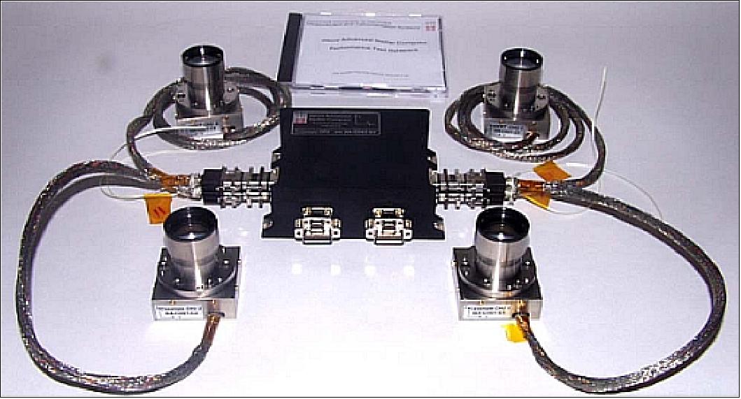
OB (Optical Bench): The purpose of the OB is the transference of the attitude from the extremely precise star trackers to the magnetometer field components. The OB ensures a highly mechanical stable platform for the magnetometer and the star trackers. A exhaustive thermo mechanical design and analysis is carried out to determine and minimize any thermal gradient that could cause a shift in the relative attitude between the two systems.
The star trackers are very magnetically clean; the separation between the two instruments (STR and VFM) is about 40 cm to reduce magnetic perturbation from the STRs. The exploitation of the symmetric system has resulted in a cylindrical tube holding the VFM sensor, minimizing transversal thermal gradients. Emphasis has been on the matching of material parameters, the use of iso-static support interfaces, and a detailed analysis of the loads. The instruments are calibrated as stand alone, and once integrated in the OB, an intercalibration and system verification is carried out to determine the relative orientation between the VFM and STR and to verify that the stability is as required.
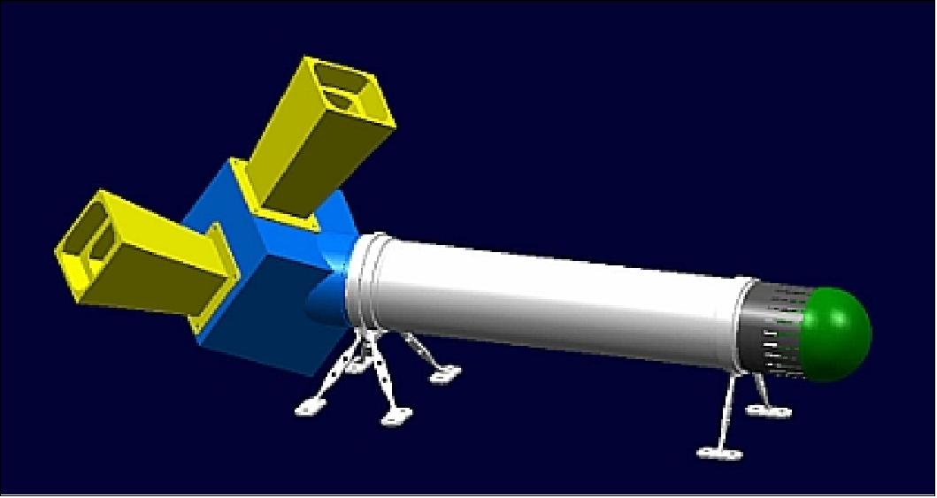
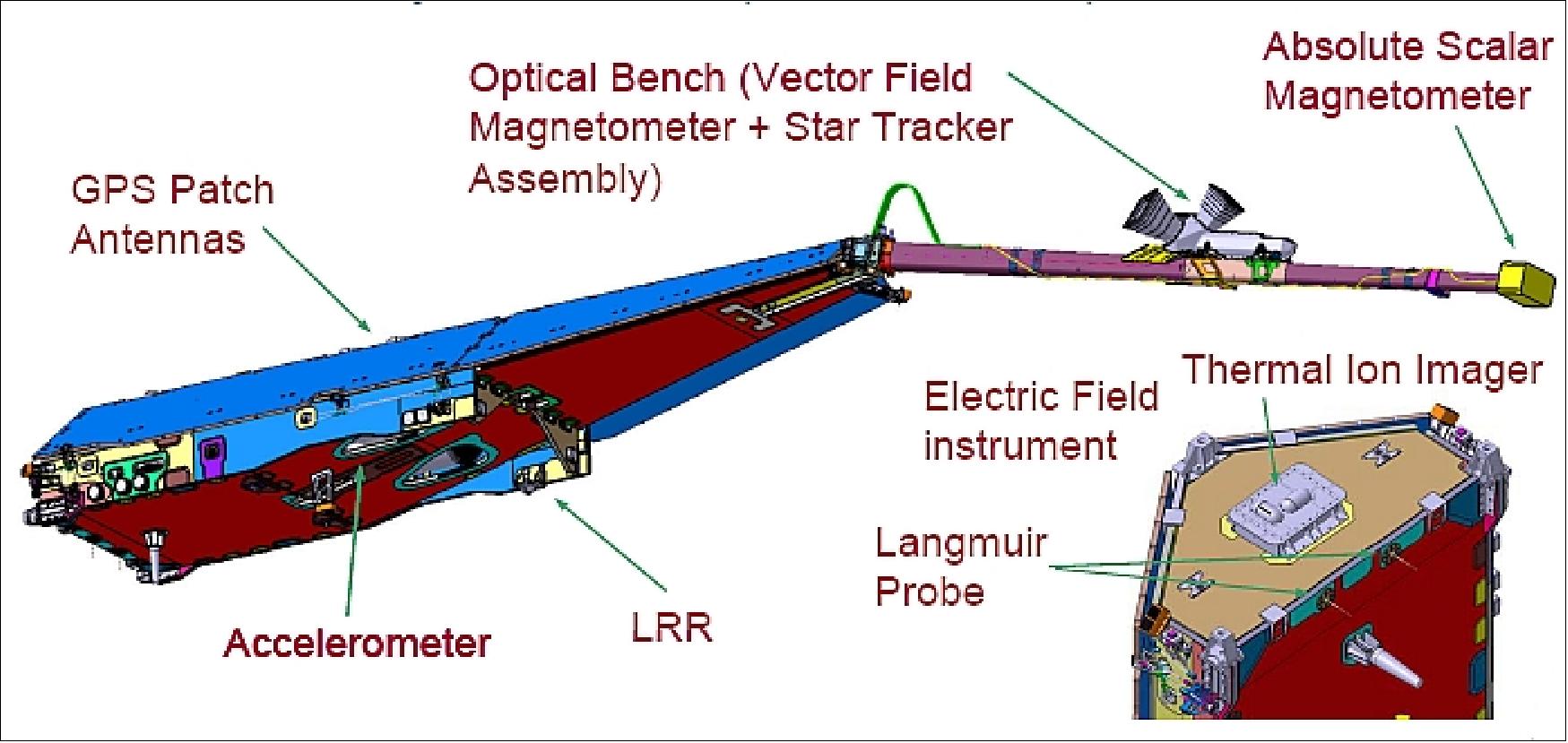
Ground Segment
The ground segment consists of the following elements: 159)
1) CDAE (Command and Data Acquisition Element), located at the Kiruna ground station, Kiruna, Sweden.
2) FOS (Flight Operations Segment), located at ESA/ESOC, Darmstadt, Germany. ESOC is in charge of monitoring and planning of satellite operations.
3) PDGS (Payload Data Ground Segment), located at ESA/ESRIN, Frascati, Italy. The main tasks of PDGS are the generation of data products from the science data, data archiving, and data distribution to the user community.
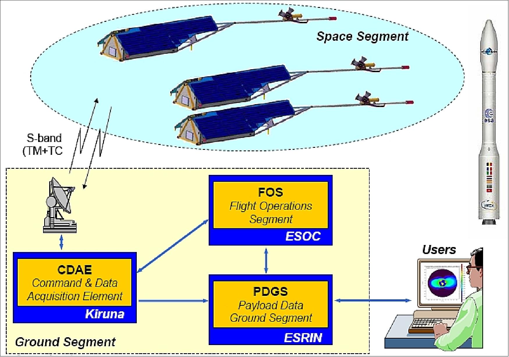
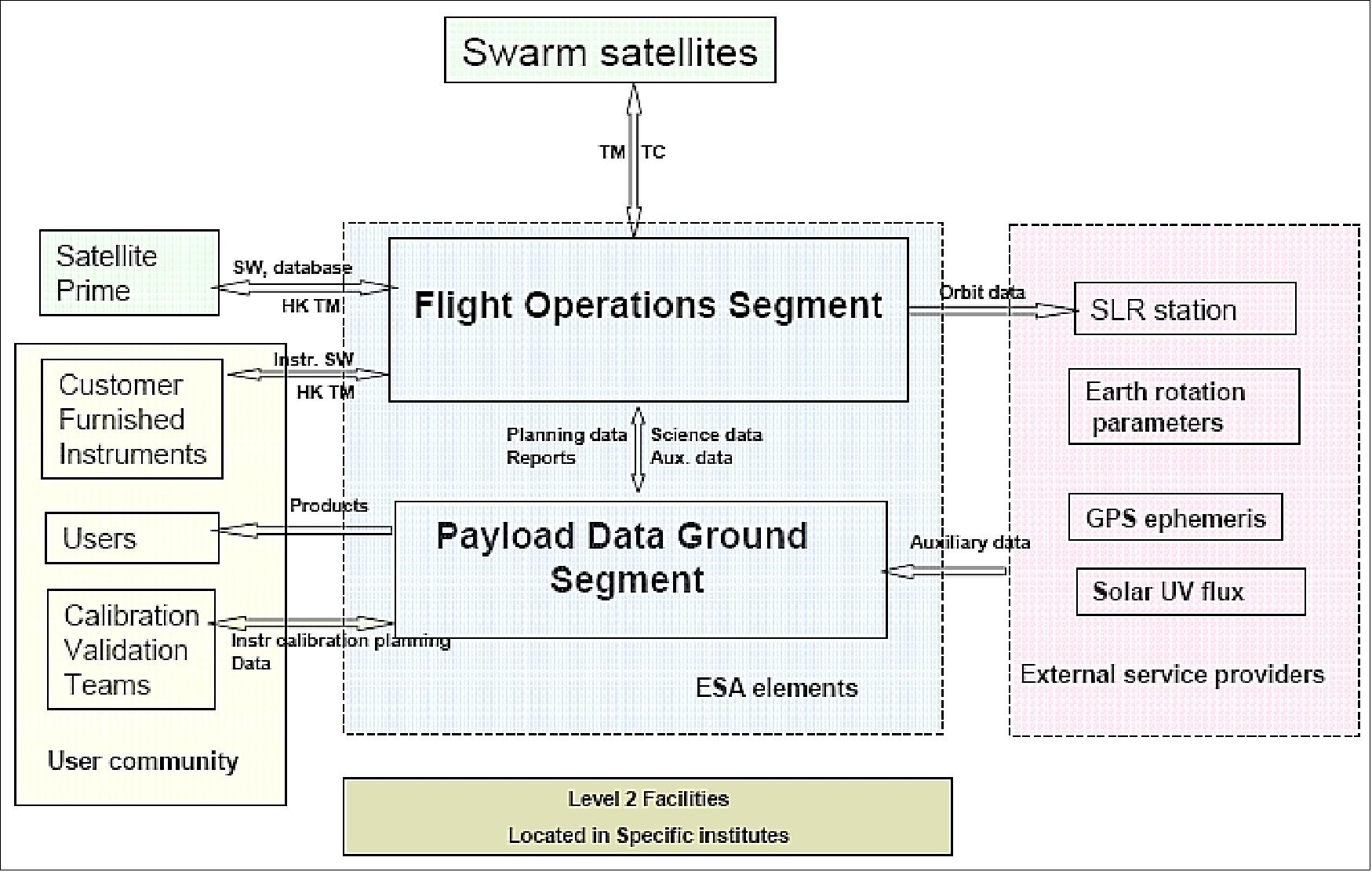
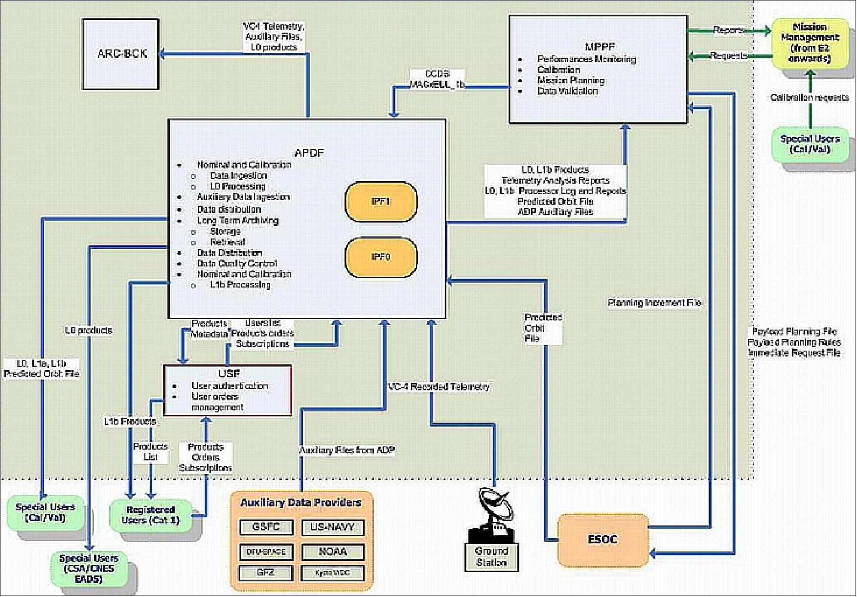
A Ground Segment for Multisatellite Operations
The concept for control of the SWARM mission during the routine phase is presented in Figure 103. It is based on the use of a single control center at ESOC, in conjunction with a prime ground station at Kiruna, augmented by external stations (Svalbard and Esrange) when required, and interconnected by a general purpose, highly available ground network. This is collectively called the FOS (Flight Operations Segment). 160)
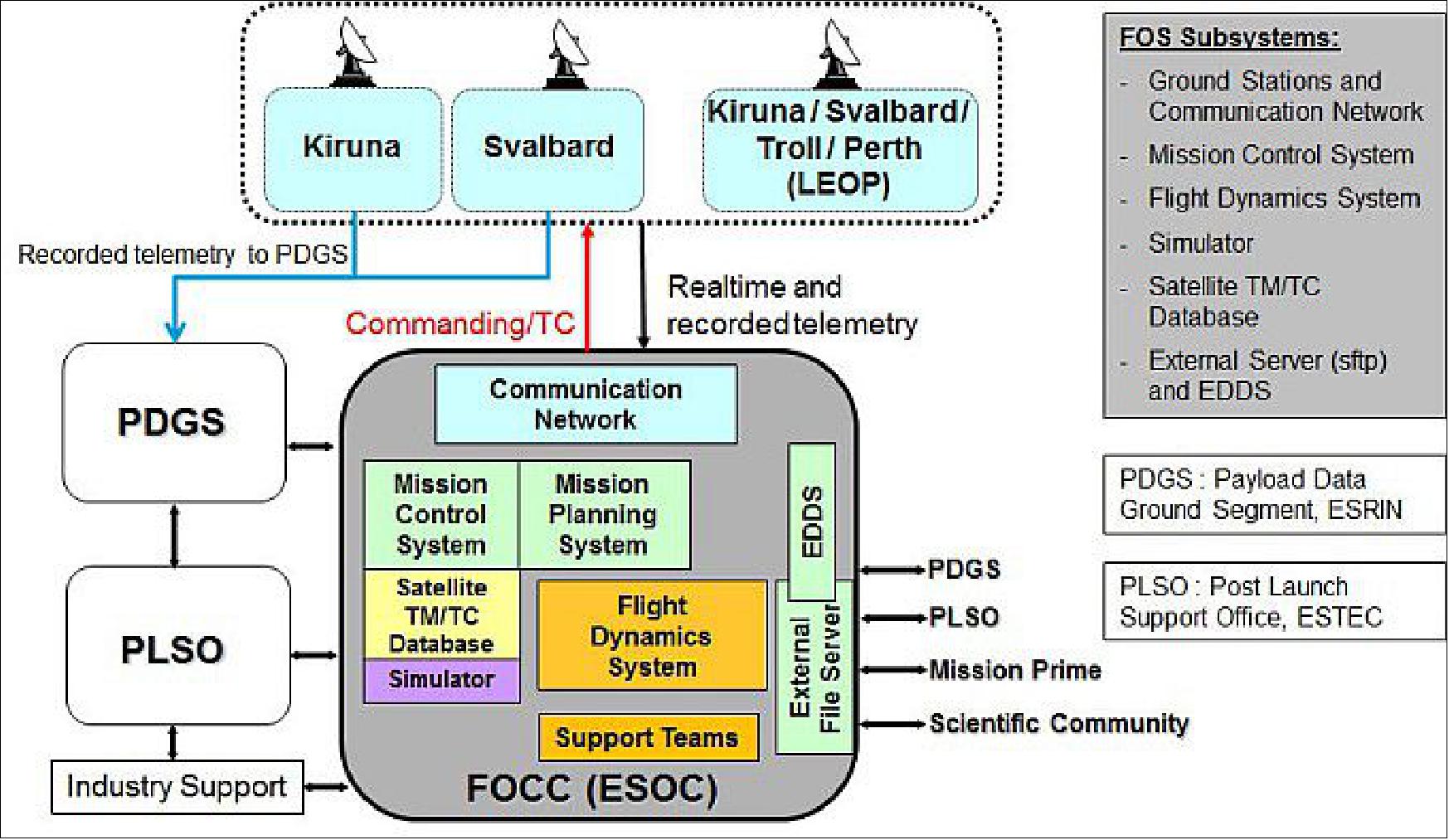
The control center, otherwise referred to as the FOCC (Flight Operations Control Center) in ESA parlance, is comprised of the following systems:
- The SWARM MCS (Mission Control System) to support, with both hardware and software, the data archiving and processing tasks essential for controlling the mission. Together with the MCS, the EDDS (EGOS Data Dissemination System) takes care of providing the Swarm data to all external interfaces.
- The SWARM MPS (Mission Planning System), supporting command request handling and the scheduling of spacecraft/payload operations.
- The FD (Flight Dynamics) System, supporting all activities related to attitude and orbit determination and prediction, preparation of slew and orbit maneuvers, spacecraft dynamics evaluation and navigation in general.
- The Spacecraft Simulator, to support procedure validation, operator training and the simulation campaign before each major phase of the mission.
Data acquired by the FOS is retrieved directly from the ground stations by the PGDS (Payload Data Ground Segment) located at ESRIN, which is in charge of processing the raw data to generate scientific products and making them available to the scientific community. Additionally, satellite housekeeping data is provided through the EDDS server to the PLSO (Post-Launch Support Office) located at ESTEC and to the spacecraft prime contractor providing industrial support.
Mission Control System and Mission Planning
The main challenge of the FOS was the multi-satellite system of Swarm, which necessitated the development of a multi-domain MCS distributed across several servers, and organized in a nominal and a backup chain. This was driven by the need for flexibility for constellation operations and parallel activities.
The Swarm MCS is based on ESOC’s generic SCOS-2000 (Spacecraft Control & Operation System-2000) infrastructure software and implements three separate domains in hardware and software, one per spacecraft, while a fourth domain handles all processes common to the three main domains. The system allows the control of the three spacecraft at the same time when required, as demonstrated during the LEOP phase, when two satellites were commanded in parallel and data was received, processed and archived for the three of them: real-time telemetry (VC0 and VC1 data streams) and recorded TM from the on-board mass memories (VC2 and VC4 data streams). In routine, only one satellite is commanded at a time, but processing of the recorded telemetry dumped during the passes may occur in parallel for the three satellites depending on the separation between spacecraft passes.
Commanding is supported by the MPS, which generates two command schedules, the SIGR (Schedule Increment Ground Schedule) and the SIOS (Schedule Increment On-Board Schedule).
The SIGR contains commands to be sent in real time and is typically related to automated pass operations by setting up the link configurations to the respective ground stations and management of the on-board mass memory (start and suspend transmission of stored data and deletion of old data).
The SIOS provides time-tagged telecommands to be loaded into the satellite MTL (Mission Timeline) on-board and mainly controls the critical data downlink strategy (transponder switch on/off, on-board statistics housekeeping, instrument mode transitions, etc.).
The default planning interval is based on seven days corresponding to a calendar week from Monday 00:00:00 UTC until Sunday 23:59:59 UTC. It is nominally prepared on Thursday of week N-1 with an execution time starting on Monday of week N and is uplinked on Friday.
All for Less: A Data Downlink Strategy
The data downlink strategy is based on just two ground station passes per satellite per day during working hours; with each pass allowing 4 to 9 minutes of commanding.
During the first pass a long data dump after the overnight out-of-coverage is performed while the second pass is a few hours after the first contact and allows to dump any remaining data that could not be retrieved during the first pass. The second pass makes the schedule more robust against outages and guarantees that the backlog is quickly recovered in case a pass is lost. It also allows recalling any data from previous passes and offers a second commanding window, which is crucial for complex payload and platform special operations that cannot be performed in a single pass.
After each pass, old data is partially deleted. This strategy ensures that always up to three days of science data (fill status of packet store up to 70%) and up to two days of housekeeping data (fill status of packet store up to 50%) are available on-board. Any data gap larger than 5 minutes detected on ground is systematically recovered by re-dumping the data. An example of the evolution of the mass memory fill level for one satellite and one week is presented in Figure 104.
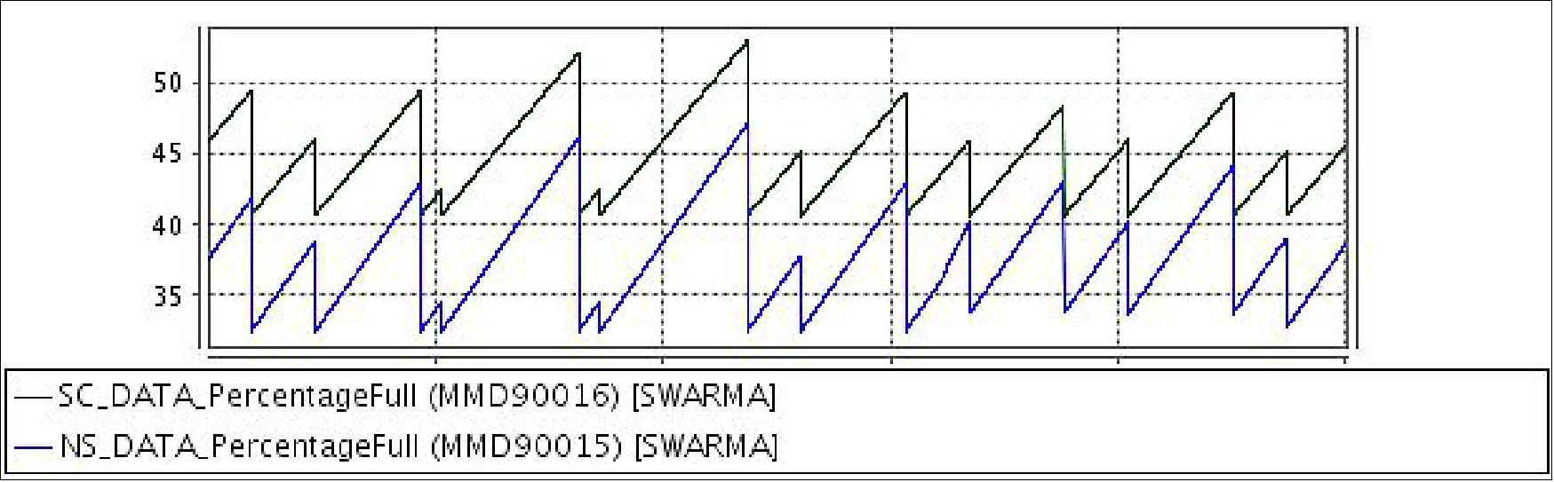
Aspects on Maneuvering the Swarm Satellite Constellation
Orbit Acquisition
The three months of commissioning in 2014 were characterized by a very tight and dynamically changing schedule of activities. All operational issues could be solved during that time, including the challenging orbit acquisition phase to achieve the final constellation.
The near polar orbit for good global coverage and regular 24 hours local time coverage about every 9 months was achieved straight away due to the nominal injection into the common separation orbit. It remained to establish the relative differences between the lower pair formed by Swarm-A/Swarm-C and the upper satellite Swarm-B. The targets in altitude and inclination difference were selected to be 50 km and 0.4º. Mainly the latter determines the relative drift rate of the LTAN (Local Time of Ascending Node) of the orbital planes between the lower pair and Swarm-B. This drift is still on-going and the LTAN difference will reach 4 hours in October 2016 and should then ideally remain within 6h ± 2h during the continuous natural decay down to 300 km until 2022 or later. To achieve this, another maneuver campaign will be needed to slow down the relative drift.
In addition, after launch the lower pair had to be separated by 5-6 minutes in LTAN and maneuvered to fly side by side with less than 10 seconds along track difference. The LTAN separation of the lower pair was achieved indirectly by performing the inclination changes of Swarm-A and Swarm-C at different times leaving, on average, six weeks in between with different nodal precession. The firing direction of the maneuvers was selected such that the semi-major axis was lowered at the same time. To achieve the required delta-v of 32m/s with the low thrust cold gas system capable of 2x0.05N, each satellite had to perform more than 130 maneuvers. The finalization of all maneuvers was completed during only 12 weeks, whereby each week was dedicated to a batch of maneuvers with a single satellite only. For each satellite a small test batch was performed to obtain a first thruster calibration. The subsequent batches consisted of 22-34 consecutive orbits with a 20 minutes maneuver around each ascending and descending node and slews in between. Here the main challenge was to come up with a robust strategy, which could be adjusted easily in case of maneuver failures and excluded any collision risk when Swarm-A approached the side-by-side configuration after completion of four additional revolutions during the six weeks drift phase. The original pre-launch maneuver plan is shown in Figure 105.
This paid off when the first Swarm-A maneuver sequence did, indeed, abort after 69% of the planned delta-v due to an on-board software problem with a shared memory address. 161)
About 36% of the loaded fuel was consumed for the orbit acquisition. This leaves enough fuel for a later maneuver campaign to slow down the relative node precession in the near future in order to stay within a LTAN difference of 6 h ±2 h. The decision about when and how far to slow down needs to be taken by the end of 2016 at the latest and requires also the best possible prediction and planning of the further decay from 440 km down to about 300 km altitude. 162)
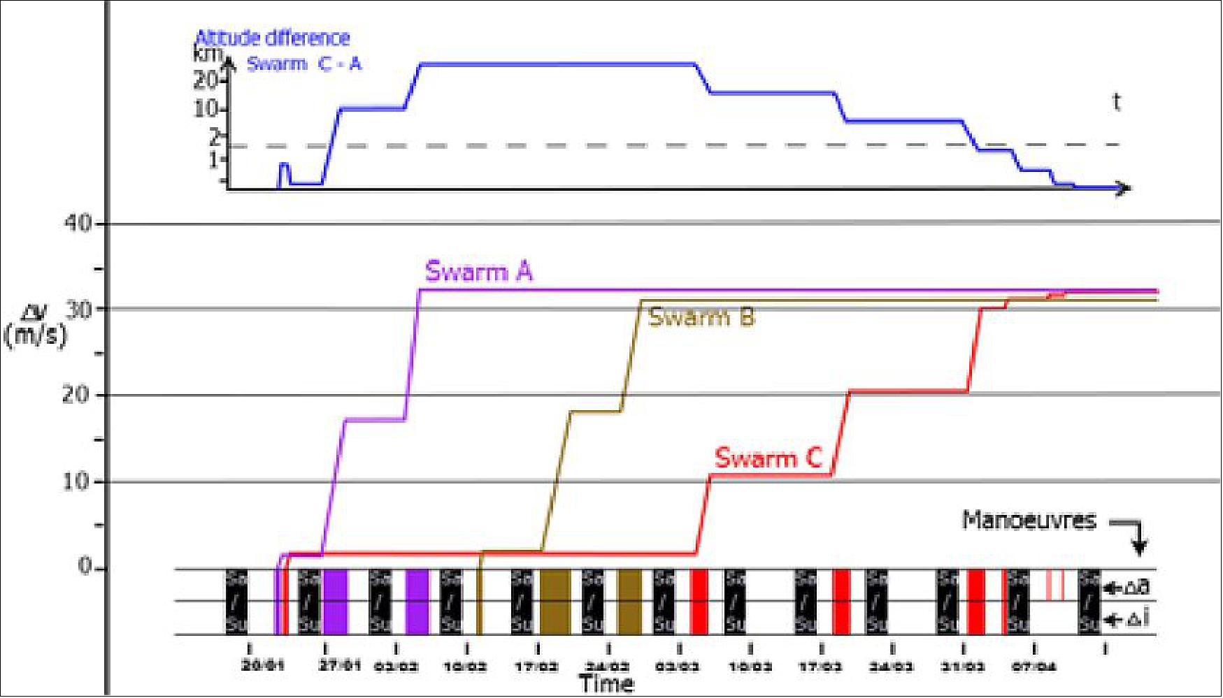
Routine and Non-routine Maneuvers
The initial orbit for the lower pair, Swarm-A and Swarm-C, was targeted at an altitude of 468 km and an inclination of 87.35 º. It is now maintained in a side-by-side constellation separated along track such that their ascending node crossing time differences are between 4 and 10 seconds. The lower limit guarantees that both spacecraft will not accidentally collide even in the case of anomalies on-board.
In addition, their eccentricity vectors are to be kept close enough to ensure an altitude difference of always less than 5 km. Also for mitigating collision risks, the eccentricities are kept as close as possible. Since the end of commissioning, 9 maneuvers on Swarm-A have been performed using a total of approximately 80 g and none on Swarm-C until now.
The other spacecraft, Swarm-B, was placed in a higher orbit (altitude circa 516 km), with an inclination higher than the lower pair by 0.4º at 87.75º. Its orbit is not controlled after the orbit acquisition phase except for necessary collision avoidance maneuvers.
Two collision avoidance maneuvers had to be executed so far, one on Swarm-B and one on Swarm-A each using around 30 g of fuel to avoid debris that endangered the safety of the satellite.
Several attitude slews were also performed to calibrate various instruments on board. Slew maneuvers were for instance performed in May 2014 to characterize the observed residuals of the two magnetometers VFM and ASM. They required careful preparation in order to ensure that they would not affect the power or thermal budget of the satellite and were compatible with the flight domain of the AOCS. Furthermore, during the routine phase the on-board fuel is spent for normal attitude maintenance (12 g per week on average).
Parameter | SWA (Swarm-A) | SWB (Swarm-B) | SWC (Swarm-C) |
Initial fuel | 105.3 | 105.0 | 102.7 |
Orbit acquisition | 38.6 | 37.7 | 38.2 |
Constellation maintenance | 0.080 | 0 | 0 |
Collision avoidance | 0.030 | 0.030 | 0 |
Normal attitude maintenance since routine phase | 1.63 | 1.23 | 1.54 |
Remaining fuel | 64.96 | 66.04 | 62.96 |
Challenges of Swarm Operations
Payload Operations
Although the actual spacecraft commissioning phase was concluded in spring 2014, the investigations for some payload instruments are still on-going.
One of the payloads of the Swarm constellation is the EFI (Electrical Field Instrument) in cooperation with the University of Calgary (UoC) in Canada and devoted to the measurement of spacecraft potential, electron temperature, ion properties and ultimately the electric field. Two Langmuir probes (LP) are used to measure the electron properties and spacecraft potential, while a Thermal Ion Imager (TII) is used to capture the plasma particles and produce 2D maps with two CCD sensors.
The intended concept of the TII was full-time operations of the imager, but, in practice, some indications of image degradation arose after a period of continuous operation depending on the satellite. Therefore, in order to maximize the scientific return, it was decided to operate the TII for just a limited and fixed number of orbits per day, in order to ensure good quality data in regions where the physical phenomena, especially at high latitudes, are of higher interest. The LPs are not affected and are always producing good quality data.
This modified concept required the need of a formal coordination between the FOS and the scientific community in order to define the times of activation: in particular a new data interface called OPF (Operations Planning File) has been defined to automatically process the inputs created by UoC and integrate them in the mission planning process at ESOC.
In parallel with the scientific measurements, several tests were carried out, mainly for Swarm-C, in order to raise the TII voltages and the temperatures of the inner instrument and to scrub possible contaminants from inside the chamber, suspected as the possible source for the image degradation. After these tests, several parameter setting updates were applied and, during the last year, the number of orbits used for science operations has successively increased, a sign of the improvement in the continuous and step-by-step fine tuning of the instrument operations. Moreover, a periodic calibration of the CCD gain maps was performed for the two sensors of each TII separately, in order to provide the conditions for good data exploitation.
Table 13 summarizes the different kind of tests performed in order to characterize the TII image anomaly. All these unforeseen activities, far beyond the original assumptions, resulted in a significant extra workload for the FCT. Large efforts were necessary to prepare, schedule and execute all the tests in a setup closer to a “extended commissioning phase” than routine operations.
Special activities performed | SWA (Swarm-A) | SWB (Swarm-B) | SWC (Swarm-C) |
CCD gain map updates | 5 | 5 | 4 |
Fixed MCP (Microchannel Plate) voltage tests | 1 | - | 6 |
Correction of AGC (Antenna Gain Control) settings | > 20 | ||
Inner dome scrubbing tests | >5 | ||
Phosphor screen voltage updates | >20 | ||
Shutter duty cycle tests | >5 | ||
The health status of the VFM (Vector Field Magnetometers) and the ASM (Absolute Scalar Magnetometers) is excellent, with the exception of the failure of both ASMs on Swarm-C just after launch (this was one of the reasons for the selection of Swarm-B as the upper satellite). The ASMs on Swarm-A and Swarm-B are routinely operated in Vector Mode and the three active VFMs are producing data at 50 Hz on the three spacecraft. Careful monitoring of temperatures, voltages, currents and other payload parameters is performed by the FCT (Flight Control Team) on a regular basis to detect any anomalous behavior.
A residual bias was identified between the measurement of the VFM and the ASM, which was presumably related to a thermal effect of the instruments. In order to characterize this behavior, Swarm-B was slewed four times by 90º. The spacecraft remained in this special attitude for 5 orbits. This operation was performed together with coordinated slews of Swarm-A and Swarm-C, four times by 90º in the reverse direction and offset by 3 orbits. The two satellites remained in each attitude position for 6 orbits.
Additional tests became also necessary for the ACC (Accelerometer) instruments on-board the Swarm satellites. The dependency of the ACC performance with respect to temperature variations appeared to be more complex than anticipated during the design phase. Tests were created in order to reduce thermal variations by using different On/Off heater strategies, in some cases with the nominal and the redundant heaters used in parallel. Those tests required careful preparation to schedule and execute more than 6000 commands synchronized with Sun eclipses.
Figure 106 shows an example of heater profile activation for one of the tests performed. The heater profiles are designed to analyze the impact of various delay activations versus start and end of eclipses in order to achieve stabilization of the ACC temperature. The tmax and tmin times closely match the entry and exit of Sun eclipses and are used as reference for the heater activation.
Test campaigns with attitude thruster activations were conducted to deduce ACC scale factors needed to adjust accelerometer deviations for all satellites. All three axes were calibrated using dedicated thruster activations designed to minimize the impact on the attitude and the orbit.
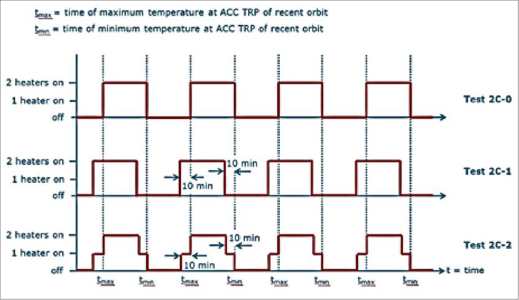
Figure 107 shows an example of the along track scale factor calibration scenario used for all Swarm satellites. It shows the impact of the thruster activations selected on the orbit and rotation of the satellite. It consisted in four separated firings designed to test along-track acceleration in both positive and negative direction and to bring the satellite back to its original position and rotation at the end of the operation. Those tests required a de-activation of the AOCS and had to be geolocalized for best performance. They, therefore, required a very careful preparation and analysis from the FCT before their execution. Currently, a six months calibration campaign is on-going to verify the stability of the scale factor over time.
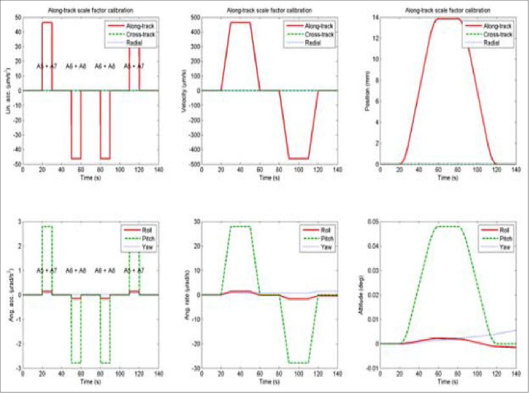
References
1) N. Olsen, R. Haagmans, T. J. Sabaka, A. Kuvshinov, S. Maus, M. E. Purucker, M. Rother, V. Lesur, M. Mandea, “The Swarm End-to-End mission simulator study: A demonstration of separating the various contributions to Earth's magnetic field using synthetic data,” Earth Planets Space, Vol. 58, 2006, pp. 359-370
2) “ESA's Magnetic Field Mission Swarm,” URL: http://www.esa.int/esaLP/ESA3QZJE43D_LPswarm_1.html
3) M. Thomsen, J. M. G. Merayo, “Data Handling System for Magnetic Nanoprobe SWARM (MAGNAS),” Proceedings of IAC 2004, Vancouver, Canada, Oct. 4-8, 2004, IAC-04-U.4.01
4) A. Schönenberg, R. Haagmans, A. Regan, A. Ginati, Y. Menard, “Swarm - Three Explorers of the Earth Magnetic Field and its Environment,” 5th IAA Symposium on Small Satellites for Earth Observation, Berlin, Germany, April 4-8, 2005
5) “A 'Swarm' of satellites for a unique look inside the Earth,” June 3, 2004, http://www.esa.int/esaCP/SEMXZH2VQUD_index_0.html
6) Y. Menard, R. Bock, E. Neri, R. Haagmans, “Swarm Mission Concept,” Proceedings of the First Swarm International Science Meeting, Nantes, France, May 3-5, 2006, WPP-261
7) http://www.esa.int/esaMI/Operations/SEM27Z8L6VE_0.html
8) E. Friis-Christensen, H. Lühr, D. Knudsen, R. Haagmans, “Swarm – An Earth Observation Mission investigating Geospace,” Advances in Space Research, Volume 41, Issue 1, 2008, pp. 210-216
9) Roger Haagmans, “ESA's supporting activities related to Mass Transport in the Earth System,” Joint GSTM and DFG SPP Symposium, GFZ Potsdam, Oct. 15-17, 2007, URL: http://www.massentransporte.de/fileadmin/20071015-17-Potsdam/mi_1410_07_haagmans.pdf
10) Max Pignède , Mario Merri, Vemund Reggestad, Peter Fritzen, Michael Irvine, “The Swarm constellation simulator - A brand new, but still operationally responsive development,” Proceedings of the Ground System Architectures Workshop (GSAW 2009), Torrance, CA, USA, March 23-26, 2009, URL: http://sunset.usc.edu/gsaw/gsaw2009/s4/pignede.pdf
11) Nils Olsen, Juliane Maries, “From Ørsted to Swarm – Challenges for exploring the Earth’s magnetic field from Space,” Nordic Space Volume 15, No 2, 2007, pp.9-12, URL: http://www.spacecenter.dk/~nio/papers/NSA188-Olsen-2007.pdf
12) Proceedings of ESA's Second Swarm International Science Meeting, June 24-26, 2009, Potsdam, Germany, URL: http://www.congrex.nl/09c24/programme.html
13) Eigil Friis-Christensen, “Scientific goals of Swarm,” Proceedings of ESA's Second Swarm International Science Meeting, June 24-26, 2009, Potsdam, Germany, WPP-303, URL: http://www.congrex.nl/09c24/S1/S1_00_Friis-Christensen_presentation.pdf
14) Yvon Menard, “Swarm Mission Status,” Proceedings of ESA's Second Swarm International Science Meeting, June 24-26, 2009, Potsdam, Germany, WPP-303, URL: http://www.congrex.nl/09c24/S1/S1_02_Menard_presentation.pdf
15) R. Haagmans, R. Bock, H. Rider, K. Fletcher, “Swarm - ESA's Magnetic Field Mission,” ESA, BR-302, October 2012, URL: http://esamultimedia.esa.int/multimedia/publications/BR-302/offline/download.pdf
16) “Swarm : Why magnetism matters,” Astrium, Oct. 4, 2013, URL: https://web.archive.org/web/20131101001634/http://www.astrium.eads.net/en/news2/why-magnetism-matters.html
17) Richard Holme, “Swarm-Near-Earth Multi-Satellite Probing of the Geomagnetic Field,” 2012 NCEO / CEOI (National Centre for Earth Observation/Centre for EO Instrumentation)Joint Science Conference, Nottingham Jubilee Campus, UK, Sept. 17-20, 2012, URL: http://www.nceo.ac.uk/assets/presentations/2012_conference_NOTTINGHAM/NCEOCONF2012_0918_Holme.pdf
18) “Swarm - The Earth's Magnetic Field and Environment Explorers,” ESA, Earth Explorers Users Consultation Meeting, 19-20 April 2004, URL: http://esamultimedia.esa.int/docs/EEUCM/Swarm_handout.pdf
19) “Magnetic Fields -- History,” NASA, URL: http://www-spof.gsfc.nasa.gov/Education/whmfield.html
20) Yvon Menard, Roger Haagmans and the Swarm Project Team, Rune Floberghagen, Juan Piñeiro, “Swarm: ESA’s magnetic field mission - A Journey to Earth's Core,” ESA Bulletin No 151, August 2012, pp.2-15, URL: https://earth.esa.int/c/document_library/get_file?folderId=131556&name=DLFE-3101.pdf
21) Jean-Michel Léger, “Spaceborne scalar magnetometers to map the Earth’s magnetic field,” CLEFS CEA, No 56 , Winter 2007-2008, URL: http://www.cea.fr/var/cea/storage/static/gb/library/Clefs56/pdf-gb/Clefs%2056_p100_102_LegerGB.pdf
22) Roger Haagmans, Gernot Plank, “Swarm: the Earth’s Magnetic Field and Environment Explorers,” URL: http://pcwww.liv.ac.uk/~holme/RAS/haagmans.pdf
23) E. F. Christensen, “Scientific Goals of Swarm,” Proceedings of the First Swarm International Science Meeting, Nantes, France, May 3-5, 2006, WPP-261
24) N. Olsen, R. Haagmans, T. J. Sabaka, A. Kuvshinov, S. Maus, M. E. Purucker, M. Rother, V. Lesur, M. Mandea, “The Swarm End-to-End mission simulator study: A demonstration of separating the various contributions to Earth's magnetic field using synthetic data,” Earth Planets Space (special issue on Swarm), Vol. 58, No 4, April 2006, pp. 359-370, URL: http://www.dsri.dk/~nio/papers/EPS_58040359.pdf
25) S. Maus., H. Lühr, M. Purucker, “Simulation of the high-degree lithospheric field recovery for the Swarm constellation of satellites,” Earth Planets Space (special issue on Swarm), Vol. 58, No 4, April 2006, pp. 397-407, URL: http://www.geomag.us/info/Smaus/Doc/swarm_e2e_Maus.pdf
26) E. Thébault, “Global lithospheric magnetic field modelling by successive regional analysis,” Earth Planets Space (special issue on Swarm), Vol. 58, No 4, April 2006, pp. 485-495, URL: http://www.terrapub.co.jp/journals/EPS/pdf/2006/5804/58040485.pdf
27) C. Manoj, A. Kuvshinov, S. Maus, H. Lühr, “Ocean circulation generated magnetic signals,” Earth Planets Space (special issue on Swarm), Vol. 58, No 4, April 2006, pp. 429-437, URL: http://www.geomag.us/info/Smaus/Doc/Manoj_EPS_swarm.pdf
28) “ESA selects new Earth-observation Missions,” May 29, 2002, URL: http://www.esa.int/esaEO/ESA87RG18ZC_index_2.html
29) “Construction of Swarm satellites to begin,” Nov. 8, 2007, URL: http://www.esa.int/esaLP/SEMQXVUOM8F_LPswarm_0.html
30) ESA's Swarm trio on its way to watch over our Planet's magnetic shiled,” ESA, Nov. 22, 2013, URL: http://www.esa.int/Our_Activities/Observing_the_Earth/The_Living_Planet_Programme/Earth_Explorers/Swarm/ESA_s_Swarm_trio_on_its_way_to_watch_over_our_planet_s_magnetic_shield
31) W. Xiang, J. L. Joergensen, “Formation Flying: A Subject Being Fast Unfolding in Space,” Proceedings of the 5th IAA Symposium on Small Satellites for Earth Observation, April 4-8, 2005, Berlin, Germany
32) Nils Olsen, Terence J. Sabaka, Luis R. Gaya-Pique, “Study of an Improved Comprehensive Magnetic Field Inversion Analysis for Swarm,” Danish National Space Center, Scientific Report 1/2007, URL: http://esamultimedia.esa.int/docs/DNSC-Scientific-Report_1_2007.pdf
33) “EADS Astrium selected for Swarm Satellites,” Nov. 17, 2005, URL: http://www.comspacewatch.com/news/viewpr.html?pid=18338
34) Albert Zaglauer, “Swarm Satellite Status,” Proceedings of ESA's Second Swarm International Science Meeting, June 24-26, 2009, Potsdam, Germany, WPP-303, URL: http://www.congrex.nl/09c24/S1/S1_01_Zaglauer_presentation.pdf
35) Carlos Pereira, Christian Oram, Cornel Boesch, Sascha Svilar, Jacques Viertl, Andreas Fix, “Comparative Development of Dimensionally Stable Structures for the Deployable Sunshield Assembly of GAIA and Composite Tube Assembly of SWARM,” Proceedings of IAC 2011 (62nd International Astronautical Congress), Cape Town, South Africa, Oct. 3-7, 2011, paper: IAC-11.C2.2.2
36) Carlos Pereira , Ian Rathband, “The Composite Tube Assembly of Swarm,” Proceedings of the 12th European Conference on Spacecraft Structures, Materials & Environmental Testing, ESA/ESTEC, Noordwijk, The Netherlands, March 20-23, 2012, SP-691
37) Thomas Usbeck, Stefan v. d. Nüll, Domenico Reggio, “The SWARM AOCS - Tailored from the CryoSat AOCS to the Specifics of a Magnetic Mission,” Proceedings of the 7th International ESA Conference on Guidance, Navigation & Control Systems (GNC 2008), June 2-5, 2008, Tralee, County Kerry, Ireland
38) Peter Zentgraf, Domenico Reggio, “Magnetic Rate Damping for Satellites in LEO,” Proceedings of the 32nd AAS Guidance and Control Conference, Breckenridge, CO, USA, Jan. 31.- Feb. 4, 2009, AAS 09-074
39) Simon Edwards, Nicholas Solway, Peter Smith, “Development of a cold gas thruster for Swarm,” Proceedings of Space Propulsion 2010, San Sebastian, Spain, May 3-6, 2010
40) Nikolaus Breier, Bernhard Kiewe, Olivier Mourra, “The Power Control and Distribution Unit for the Swarm Satellites,” Proceedings of the 8th European Space Power Conference, Constance, Germany, Sept. 14-19, 2008, ESA SP-661, Sept. 2008
41) “Satellites packed like sardines,” ESA, Nov. 8, 2013, URL: http://www.esa.int/Our_Activities/Observing_the_Earth/Swarm/Satellites_packed_like_sardines
42) Paul McMahon, Hans-Juergen Jung, Jeff Edwards, “Swarm Deployable Boom Assembly (DBA) Development of a Deployable Magnetometer Boom for the swarm Spacecraft,” Proceedings of the 15th ESMATS (European Space Mechanisms and Tribology Symposium) 2013, Noordwijk, The Netherlands, Sept. 25-27, 2013, ESA, SP-718, URL: http://www.esmats.eu/esmatspapers/pastpapers/pdfs/2013/mcmahon.pdf
43) “ESA’s Swarm trio on its way to watch over our planet’s magnetic shield,” ESA, Nov. 22, 2013, URL: http://www.esa.int/Our_Activities/Observing_the_Earth/Swarm/ESA_s_Swarm_trio_on_its_way_to_watch_over_our_planet_s_magnetic_shield
44) “Swarm Satellites Launched Successfully,” Eurockot, Nov. 22, 2013, URL: http://www.eurockot.com/2013/11/swarm-satellites-launched-successfully/
45) “SWARM – Earth's magnetic field to be accurately measured by three European satellites flying in formation,” DLR, Nov. 22, 2013, URL: http://www.dlr.de/dlr/en/desktopdefault.aspx/tabid-10081/151_read-8817/year-all/#gallery/13060
46) “Satellite trio to explore the Earth's magnetic field,” Space Daily, Nov. 27, 2013, URL: http://www.spacedaily.com/reports/Satellite_trio_to_explore_the_Earths_magnetic_field_999.html
47) Marie-Helene Thibeault, “University of Calgary technology part of European Space Agency mission launched into space,” University of Calgary, Nov. 22, 2013, URL: http://www.ucalgary.ca/utoday/issue/2013-11-22/university-calgary-technology-part-european-space-agency-mission-launched-space
48) “Swarm Mission Control ready for Tripple Launch,” ESA, Nov. 19, 2013, URL: http://www.esa.int/Our_Activities/Operations/Swarm_mission_control_ready_for_triple_launch
49) “Preparing to launch Swarm,” ESA, Sept. 13, 2013, URL: http://www.esa.int/Our_Activities/Observing_the_Earth/The_Living_Planet_Programme/Earth_Explorers/Swarm/Preparing_to_launch_Swarm
50) “Eurockot to launch two ESA Earth observation missions,” ESA, April 9, 2010, URL: http://www.esa.int/esaEO/SEM2GI0OK7G_index_0.html
51) Peter Freeborn, York Viertel, Anna Zorina, “Meeting the Future Launch Demand for Earth Observation Missions,” 8th IAA (International Academy of Astronautics) Symposium on Small Satellites for Earth Observation, Berlin, Germany, April 4-8, 2011; URL of presentation, IAA-B8-0501, http://media.dlr.de:8080/erez4/erez?cmd=get&src=os/IAA/archiv8/Presentations/IAA-B8-0501.pdf
52) “Swarm constellation heads north,” ESA, Feb. 17, 2012, URL: http://www.esa.int/esaEO/SEMBHGZXHYG_index_0.html
53) Peter Freeborn, York Viertel, “Eurockot launch services for ESA Earth observation swarm satellites,” Proceedings of the 63rd IAC (International Astronautical Congress), Naples, Italy, Oct. 1-5, 2012, paper: IAC-12-D2.2.10
54) Nils Olsen and the Swarm Mission Simulator Team, “Swarm Magnetic Field Models and Other Derived Data Products,” IAGA 2005, Toulouse. France, July 19, 2005, URL: http://www.geos.ed.ac.uk/research/geospace/presentations/pub_store/serial110.pdf
55) “Swarm: magnetic field satellites get their bearings,” ESA, Oct. 27, 2011, URL: http://www.esa.int/esaEO/SEMLV3HURTG_index_0.html
56) Detlef Sieg, Francesco Petrucciani, Gerald Ziegler, ”Swarm Flight Dynamics Operations Experiences and Mission Analysis,” Fourth Swarm Science Meeting & Geodetic Missions Workshop, Banff, Alberta, Canada, March 20-24, 2017, Presentation provided by Detlef Sieg
57) ”Swarm dodges collision during climb to escape Sun’s wrath,” ESA Space Safety, 14 July 2022, URL: https://www.esa.int/Space_Safety/Swarm_dodges_collision_during_climb_to_escape_Sun_s_wrath
58) ”Swarm unveils magnetic waves deep down,” ESA Applications, 23 May 2022, URL: https://www.esa.int/Applications/Observing_the_Earth/FutureEO/Swarm/Swarm_unveils_magnetic_waves_deep_down
59) Nicolas Gillet, Felix Gerick, Dominique Jault, Tobias Schwaiger, Julien Aubert, Mathieu Istas, ”Satellite magnetic data reveal interannual waves in Earth’s core,” PNAS, Vol. 119, No13, March 21, 2022, https://doi.org/10.1073/pnas.2115258119
60) ”Swarm and Cluster get to the bottom of geomagnetic storms,” ESA Applications, 15 December 2021, URL: https://www.esa.int/Applications/Observing_the_Earth/Swarm/Swarm_and_Cluster_get_to_the_bottom_of_geomagnetic_storms
61) Dong Wei, Malcolm W. Dunlop, Junying Yang, Xiangcheng Dong, Yiqun Yu, Tieyan Wang, ”Intense dB/dt Variations Driven by Near-Earth Bursty Bulk Flows (BBFs): A Case Study,” Geophysical Research Letters, Volume48, Issue4 , 28 February 2021, e2020GL091781, First published: 20 January 2021, https://doi.org/10.1029/2020GL091781
62) ”Swarm yields new insight into animal migration,” ESA Applications, 9 July 2021, URL: https://www.esa.int/Applications/Observing_the_Earth/Swarm/Swarm_yields_new_insight_into_animal_migration
63) Fernando Benitez-Paez, Vanessa da Silva Brum-Bastos, Ciarán D. Beggan, Jed A. Long & Urška Demšar, ”Fusion of wildlife tracking and satellite geomagnetic data for the study of animal migration,” Movement Ecology, Volume 9, Article No 31, Published: 11 June 2021, https://doi.org/10.1186/s40462-021-00268-4, URL: https://movementecologyjournal.biomedcentral.com/track/pdf/10.1186/s40462-021-00268-4.pdf
64) ”The curious incident of Swarm and sprites in the night-time,” ESA Applications, 18 May 2021, URL: https://www.esa.int/Applications/Observing_the_Earth/Swarm/The_curious_incident_of_Swarm_and_sprites_in_the_night-time
65) M. Strumik, J. Slominski, E. Slominska, J. Mlynarczyk, J. Blecki, R. Haagmans, A. Kulak, M. Popek, K. Martynski, R. Wronowski, ”Experimental Evidence of a Link Between Lightning and Magnetic Field Fluctuations in the Upper Ionosphere Observed by Swarm,” Geophysical Research Letters, Volume48, Issue4, 28 February 2021, e2020GL091507, https://doi.org/10.1029/2020GL091507, URL: https://agupubs.onlinelibrary.wiley.com/doi/epdf/10.1029/2020GL091507
66) ”Antarctica’s magnetic link to ancient neighbors,” ESA Applications, 9 March 2021, URL: https://www.esa.int/Applications/Observing_the_Earth/Swarm/Antarctica_s_magnetic_link_to_ancient_neighbours
67) Jörg Ebbing, Yixiati Dilixiati, Peter Haas, Fausto Ferraccioli & Stephanie Scheiber-Enslin, ”East Antarctica magnetically linked to its ancient neighbors in Gondwana,” Nature Journal Scientific Reports, Volume 11, Article No 5513, Published: 09 March 2021, https://doi.org/10.1038/s41598-021-84834-1
68) ”Energy from solar wind favors the north,” ESA Applications, 12 January 2021, URL: https://www.esa.int/Applications/Observing_the_Earth/Swarm/Energy_from_solar_wind_favours_the_north
69) P. Pakhotin, I. R. Mann, K. Xie, J. K. Burchill & D. J. Knudsen, ”Northern preference for terrestrial electromagnetic energy input from space weather,” Nature Communications, Volume 12, Article No 199, Published: 08 January 2021, https://doi.org/10.1038/s41467-020-20450-3,
70) Mara Johnson-Groh and Jessica Merzdorf, ”NASA Researchers Track Slowly Splitting 'Dent' in Earth’s Magnetic Field,” NASA Feature, 17 August 2020, URL: https://www.nasa.gov/feature/nasa-researchers-track-slowly-splitting-dent-in-earth-s-magnetic-field
71) ”Swarm probes weakening of Earth’s magnetic field,” ESA / Applications / Observing the Earth / Swarm, 20 May 2020, URL: http://www.esa.int/Applications/Observing_the_Earth/Swarm/Swarm_probes_weakening_of_Earth_s_magnetic_field
72) ”Magnetic north and the elongating blob,” ESA / Applications / Observing the Earth / Swarm, 14 May 2020, URL: http://www.esa.int/Applications/Observing_the_Earth/Swarm/Magnetic_north_and_the_elongating_blob
73) ”Steve over the picket fence,” ESA / Applications / Observing the Earth / Swarm, 27 November 2019, URL: http://www.esa.int/Applications/Observing_the_Earth/Swarm/Steve_over_the_picket_fence
74) W. E. Archer, J.-P. St.- Maurice, B. Gallardo-Lacourt, G. W. Perry, C. M. Cully,E. Donovan,D. M. Gillies,R. Downie,J. Smith, and D. Eurich, ”The Vertical Distribution of the Optical Emissions of a Steve and Picket Fence Event,” Geophysical Research Letters, Vol. 46, 10,719–10,725, Published online: 11 October 2019, URL: https://agupubs.onlinelibrary.wiley.com/doi/epdf/10.1029/2019GL084473
75) ”Swarm helps explain Earth’s magnetic jerks,” ESA, 01 May 2019, URL: http://www.esa.int/Our_Activities/Observing_the_Earth/Swarm/Swarm_helps_explain_Earth_s_magnetic_jerks
76) Julien Aubert & Christopher C. Finlay, ”Geomagnetic jerks and rapid hydromagnetic waves focusing at Earth’s core surface,” Nature Geoscience, Vol. 12, pp: 393-398, Published: 22 April 2019, https://doi.org/10.1038/s41561-019-0355-1
77) ”Scientists discover what powers celestial phenomenon STEVE,” AGU (American Geophysical Union), 25 April 2019, URL: https://news.agu.org/press-release/scientists-discover-what-powers-celestial-phenomenon-steve/
78) ”Swarm helps pinpoint new magnetic north for smartphones,” ESA 8 February 2019, URL: http://www.esa.int/Our_Activities/Observing_the_Earth/Swarm/Swarm_helps_pinpoint_new_magnetic_north_for_smartphones
79) ”Satellite ‘compasses’ open new window on space weather,” ESA, 7 November 2018, URL: http://m.esa.int/Our_Activities/Space_Engineering_Technology/Satellite_compasses_open_new_window_on_space_weather
80) ”ESA's unexpected fleet of space weather monitors,” ESA, 28 June 2018, URL: http://www.esa.int/Our_Activities/Preparing_for_the_Future/Discovery_and_Preparation/ESA_s_unexpected_fleet_of_space_weather_monitors
81) URL: https://earth.esa.int/web/guest/missions/esa-operational-eo-missions/swarm
82) ”Swarm turns to whistlers and storms,” ESA, 13 April, 2018, URL: http://m.esa.int/Our_Activities/Observing_the_Earth/Swarm/Swarm_turns_to_whistlers_and_storms
83) ”Electric nature,” ESA, 12 April 2018, URL: http://m.esa.int/spaceinimages/Images/2018/04/Electric_nature
84) ”St. Patrick's Day Storm,” URL: http://m.esa.int/spaceinvideos/Videos/2018/04/St._Patrick_s_Day_storm
85) ”Magnetic lithosphere detailed,” ESA, 10 April 2018, URL: http://m.esa.int/spaceinvideos/Videos/2018/04/Magnetic_lithosphere_detailed
86) ”Swarm tracks elusive ocean magnetism,” ESA, 10 April 2018, URL: http://m.esa.int/Our_Activities/Observing_the_Earth/Swarm/Swarm_tracks_elusive_ocean_magnetism
87) ”Getting to know Steve,” ESA, 16 March, 2018, URL: http://m.esa.int/Our_Activities/Observing_the_Earth/Swarm/Getting_to_know_Steve
88) Jacey Fortin, ”That Ghostly, Glowing Light Above Canada? It’s Just Steve,” The New York Times, 25 April 2018, URL: https://www.nytimes.com/2017/04/25/science/aurora-borealis-steve.html
89) Elizabeth A. MacDonald, Eric Donovan, Yukitoshi Nishimura, Nathan A. Case, D. Megan Gillies, Bea Gallardo-Lacourt, William E. Archer, Emma L. Spanswick, Notanee Bourassa, Martin Connors, Matthew Heavner, Brian Jacke, Burcu Kosar, David J. Knudsen, Chris Ratzlaff, Ian Schofield, ”New science in plain sight: Citizen scientists lead to the discovery of optical structure in the upper atmosphere,” Science Advances,” Vol. 4, No. 3, 02 March 2018, URL: http://advances.sciencemag.org/content/advances/4/3/eaaq0030.full.pdf
90) T. N. Davis, ”Observed characteristics of auroral forms,” Space Science Review, Vol. 22, 77–113 (1978)
91) C. W. Unick, E. Donovan, M. Connors, B. Jackel, ”A dedicated H-beta meridian scanning photometer for proton aurora measurement,” Journal of Geophysical Research, Space Physics, Vol. 122, pp: 753–764, 2017
92) ”Swarm trio becomes a quartet,” ESA, 22 Feb. 2018, URL: http://m.esa.int/Our_Activities/Observing_the_Earth/Swarm/Swarm_trio_becomes_a_quartet
93) ”Swarm details energetic coupling,” ESA, 15 Feb. 2018, URL: http://m.esa.int/Our_Activities/Observing_the_Earth/Swarm/Swarm_details_energetic_coupling
94) Ryan M. McGranaghan, Anthony J. Mannucci , Colin Forsyth, ”A Comprehensive Analysis of Multiscale Field-Aligned Currents: Characteristics, Controlling Parameters, and Relationships,” Journal of Geophysical Research: Space Physics, Vol. 122, pp: 11,931–11,960, https://doi.org/10.1002/2017JA024742, Published online 5 Dec. 2017, URL: http://onlinelibrary.wiley.com/doi/10.1002/2017JA024742/epdf
95) ”Swarm celebrates its 4th anniversary in space,” ESA, 22 November 2017, URL: https://earth.esa.int/web/guest/missions/esa-eo-missions/swarm/results-news/-/article/swarm-celebrates-its-fourth-anniversary-in-space
96) ”ESA Member States approve Swarm extension,” ESA, 20 Nov. 2017, URL: https://web.archive.org/web/20180105233555/https://earth.esa.int/web/guest/missions/esa-eo-missions/swarm/operational-news/-/article/esa-member-states-approve-swarm-extension
97) Information provided by Nils Olsen on June 22, 2017
98) ”When Swarm met Steve,” ESA, April 21, 2017, URL: http://www.esa.int/Our_Activities/Observing_the_Earth/Swarm/When_Swarm_met_Steve
99) Elia Maestroni, Ignacio Clerigo, Frank-Jürgen Diekmann, ”Three Times Three: Three Years of Swarm Routine Operations and Beyond,” Fourth Swarm Science Meeting & Geodetic Missions Workshop, Banff, Alberta, Canada, March 20-24, 2017, The ”poster presentation” was provided by Elia Maestroni of ESA/ESOC, Darmstadt, Germany.
100) ”Supersonic plasma jets discovered,” ESA, March 23, 2017, URL: http://m.esa.int/Our_Activities/Observing_the_Earth/Swarm/Supersonic_plasma_jets_discovered
101) ”Swarm detects asymmetry,” ESA, March 22, 2017, URL: http://m.esa.int/Our_Activities/Observing_the_Earth/Swarm/Swarm_detects_asymmetry
102) ”Unravelling Earth’s magnetic field,” ESA, March 21, 2017, URL: http://m.esa.int/Our_Activities/Observing_the_Earth/Swarm/Unravelling_Earth_s_magnetic_field
103) ”Anatomy of a debris incident,” ESA, Feb. 1, 2017, URL: http://m.esa.int/Our_Activities/Operations/Anatomy_of_a_debris_incident
104) ”There’s a jet stream in our core,” ESA, Dec. 19, 2016, URL: http://m.esa.int/Our_Activities/Observing_the_Earth/Swarm/There_s_a_jet_stream_in_our_core
105) Philip W. Livermore, Rainer Hollerbach, Christopher C. Finlay, ”An accelerating high-latitude jet in Earth’s core,” Nature Geoscience, Dec. 19, 2016, doi:10.1038/ngeo2859
106) ”Swarm reveals why satellites lose track,” ESA, Oct. 28, 2016, URL: http://m.esa.int/Our_Activities/Observing_the_Earth/Swarm/Swarm_reveals_why_satellites_lose_track
107) Chao Xiong, Claudia Stolle, Hermann Lühr, ”The Swarm satellite loss of GPS signal and its relation to ionospheric plasma irregularities,” Space Weather, Volume 14, Issue 8, August 13, 2016, pp: 563–577, DOI: 10.1002/2016SW001439, URL of abstract: http://onlinelibrary.wiley.com/doi/10.1002/2016SW001439/abstract
108) ”Magnetic oceans and electric Earth,” ESA, Oct. 3, 2016, URL: http://m.esa.int/Our_Activities/Observing_the_Earth/Swarm/Magnetic_oceans_and_electric_Earth
109) Alexander V. Grayver, Neesha R. Schnepf, Alexey V. Kuvshinov, Terence J. Sabaka, Chandrasekharan Manoj, Nils Olsen, ”Satellite tidal magnetic signals constrain oceanic lithosphere-asthenosphere boundary,” Science Advances, 30 Sept. 2016: Vol. 2, no. 9, e1600798, DOI: 10.1126/sciadv.1600798, URL: http://advances.sciencemag.org/content/advances/2/9/e1600798.full.pdf
110) N. R. Schnepf, A. Kuvshinov, T. Sabaka, ”Can we probe the conductivity of the lithosphere and upper mantle using satellite tidalmagnetic signals?,” Geophysical Research Letters, Vol. 42, article online 8 APR 2015, doi:10.1002/2015GL063540, URL: https://www.ethz.ch/content/dam/ethz/special-interest/erdw/geophysics/epm-dam/images/Tides/Schnepf_Kuvshinov_Sabaka_2015_GRL.pdf
111) Detlef Sieg, Frank Diekmann, ”Options for Further Orbit Evolution of the Swarm Mission,” Proceedings of the Living Planet Symposium 2016, Prague, Czech Republic, May 9-13, 2016 (ESA SP-740, August 2016)
112) Earth's magnetic heartbeat,” ESA, May 10, 2016, URL: http://www.esa.int/Our_Activities/Observing_the_Earth/Swarm/Earth_s_magnetic_heartbeat
113) ”Swarm constellation,” ESA, >Oct. 15, 2013, URL: http://www.esa.int/spaceinimages/Images/2013/10/Swarm_constellation
114) ”Swarm ASM-VFM Residual dataset,” ESA, Dec. 22, 2015, URL: https://earth.esa.int/web/guest/missions/esa-operational-eo-missions/swarm/news
115) ”Programs in Progress - Status at end of July 2015 -Swarm,” ESA Bulletin No 163, 3rd quarter 2015, pp: 57-58, URL: http://esamultimedia.esa.int/multimedia/publications/ESA-Bulletin-163/offline/download.pdf
116) “Magnetic complexity begins to untangle,” ESA, June 22, 2015, URL: http://www.esa.int/Our_Activities/Observing_the_Earth/Swarm/Magnetic_complexity_begins_to_untangle
117) P. Alken, S. Maus, A. Chulliat, P. Vigneron, O. Sirol,G. Hulot, “Swarm equatorial electric field chain: First results,” Geophysical Research Letters, Volume 42, Issue 3,16 February 2015, pp: 673–680, doi: 10.1002/2014GL062658
118) Hermann Lühr, Jaeheung Park, Jesper W. Gjerloev, Jan Rauberg, Ingo Michaelis, Jose M. G. Merayo, Peter Brauer, “Field‐aligned currents' scale analysis performed with the Swarm constellation,” Geophysical Research Letters, Volume 42, Issue 1, 16 January 2015, pp: 1–8, doi: 10.1002/2014GL062453
119) A. Spicher, T. Cameron, E. M. Grono, K. N. Yakymenko, S. C. Buchert, L. B. N. Clausen, D. J. Knudsen, K. A. McWilliams, J. I. Moen, “Observation of polar cap patches and calculation of gradient drift instability growth times: A Swarm case study,” Geophysical Research Letters, Volume 42, Issue 2, 28 January 2015, pp: 201–206, doi: 10.1002/2014GL062590
120) Gauthier Hulot, Pierre Vigneron, Jean‐Michel Léger, Isabelle Fratter, Nils Olsen, Thomas Jager, François Bertrand, Laura Brocco, Olivier Sirol, Xavier Lalanne,Axel Boness, Viviane Cattin, “Swarm's absolute magnetometer experimental vector mode, an innovative capability for space magnetometry,” Geophysical Research Letters, Volume 42, Issue 5, 16 March 2015, pp: 1352–1359, doi: 10.1002/2014GL062700
121) ESA Bulletin No 161, May 11, 2015, p. 74, URL: http://esamultimedia.esa.int/multimedia/publications/ESA-Bulletin-161/offline/download.pdf
122) Nils Olsen, Gauthier Hulot, Vincent Lesur, Christopher C. Finlay, Ciaran Beggan, Arnaud Chulliat, Terence J. Sabaka, Rune Floberghagen, Eigil Friis-Christensen, Roger Haagmans, Stavros Kotsiaros, Hermann Lühr, Lars Tøffner-Clausen, Pierre Vigneron, “The Swarm Initial Field Model for the 2014 geomagnetic field,” Geophysical Research Letters, Vol. 42, doi:10.1002/2014GL062659.URL: ftp://ftp.space.dtu.dk/pub/cfinl/publications/2015_Olsen_Hulot_Lesur_Finlay_etal.pdf
123) “Swarm celebrates one year in orbit,” ESA, Nov. 24, 2014, URL: https://earth.esa.int/web/guest/missions/esa-operational-eo-missions/swarm/news/-/article/swarm-celebrates-one-year-in-orbit
124) “Swarm,” ESA Bulletin, No 160, November 2014, p. 73
125) Isabelle Fratter, Jean-Michel Leger, Francois Bertrand, Thomas Jager, Gauthier Hulot, Laura Brocco, Pierre Vigneron, “Swarm Absolute Scalar Magnetometers first in-orbit results,” Proceedings of the 65th International Astronautical Congress (IAC 2014), Toronto, Canada, Sept. 29-Oct. 3, 2014, paper: IAC-14,B1,3.1
126) “Swarm reveals Earth's changing magnetism,” ESA, June 19, 2014, URL: http://www.esa.int/Our_Activities/Observing_the_Earth/Swarm/Swarm_reveals_Earth_s_changing_magnetism
127) “Earth’s ever-changing magnetic field,” ESA, June 19,2014, URL: http://www.esa.int/spaceinvideos/Videos/2014/06/Earth_s_ever-changing_magnetic_field
128) “Swarm's precise sense of magnetism,” ESA, May 7, 2014, URL: http://www.esa.int/Our_Activities/Observing_the_Earth/Swarm/Swarm_s_precise_sense_of_magnetism
129) R. Mackenzie, R. Bock, D. Kuijper, P. Ramos-Bosch, D. Sieg, G. Ziegler, ”A Review of Swarm Flight Dynamics Operations from launch to routine phase,” Proceedings of 24th International Symposium on Space Flight Dynamics, Laurel, Maryland, USA, 5 - 9 May, 2014, URL: http://issfd.org/ISSFD_2014/ISSFD24_Paper_S14-4_Mackenzie.pdf
130) “Swarm heads for new heights,” ESA, Feb. 6, 2014, URL: http://www.esa.int/Our_Activities/Observing_the_Earth/Swarm/Swarm_heads_for_new_heights
131) “End of the beginning for Swarm Trio,” ESA, Nov. 26, 2013, URL: http://www.esa.int/Our_Activities/Operations/End_of_the_beginning_for_Swarm_trio
132) J. M. G. Merayo, J. L. Jørgensen, E. Friis-Christensen, P. Brauer, F. Primdahl, P. S. Jørgensen, T. H. Allin, T. Denver, “The Swarm Magnetometry Package,” Proceedings of the 6th IAA Symposium on Small Satellites for Earth Observation, Berlin, Germany, April 23 - 26, 2007
133) “Swarm - The Earth's Magnetic Field and Environment Explorers Technical and Programmatic Annex,” ESA, Annex to ESA SP-1279(6) April 2004, URL: http://esamultimedia.esa.int/docs/EEUCM/SWARM_TPA.pdf
134) Peter S. Jørgensen, José Merayo, John L. Jørgensen, “Pre-Flight Calibration of the Swarm Vector Magnetometer Package,” Proceedings of ESA's Second Swarm International Science Meeting, June 24-26, 2009, Potsdam, Germany, WPP-303, URL: http://www.congrex.nl/09c24/S1_Posters/S1_P01_Jorgensen_paper.pdf
135) Jose M. G. Merayo, “The Vector Field Magnetometer (VFM) on Swarm,” Proceedings of ESA's Second Swarm International Science Meeting, June 24-26, 2009, Potsdam, Germany, WPP-303
136) Jos é M. G. Merayo, John L. Jørgensen, Eigil Friis-Christensen, Peter Brauer, Fritz Primdahl, Peter S. Jørgensen, Thomas H. Allin, Troelz Denver, “The Swarm Magnetometry Package,” Springer Netherlands, April 2008, ISBN: 978-1-4020-6942-0
137) http://smsc.cnes.fr/SWARM/GP_instrument.htm
138) http://smsc.cnes.fr/SWARM/Instr_Descript_Archi.pdf
139) http://smsc.cnes.fr/SWARM/ASM_Principle.pdf
140) Jean-Michel Leger , François Bertrand, Thomas Jager, Matthieu Le Prado, Isabelle Fratter, Jean-Claude Lalaurie, “Swarm absolute scalar and vector magnetometer based on helium 4 optical pumping,” Proceedings of ESA's Second Swarm International Science Meeting, June 24-26, 2009, Potsdam, Germany, WPP-303, URL: http://www.congrex.nl/09c24/S1/S1_05_Leger_paper.pdf
141) W. Fourcault, J-M. Léger, V. Costes, I. Fratter, L. Mondin, “Athermal Fiber Laser for the Swarm Absolute Scalar Magnetometer,” ICSO 2010 (International Conference on Space Optics), Rhodes Island, Greece, Oct. 4-8, 2010, URL: http://smsc.cnes.fr/SWARM/PDF/LEGER_ICSO_PAPER.pdf
142) Isabelle Fratter, Jean-Michel Léger, François Bertrand, Thomas Jager, Matthieu Le Prado, William Fourcault, “Development and Space Qualification of the Swarm Absolute Scalar Magnetometer,” IEEE sensors 2010, Waikoloa, HI, USA, Nov. 1-4, 2010, paper No 1291, URL: http://smsc.cnes.fr/SWARM/PDF/Sensors2010_paper_1291_FRATTER_2_IEEE.pdf
143) D. Ramecourt, T. Guettler Sergeant, T. Buret, C. Rougane, I. Fratter, D. Veyrié, O. Gilard, V. Costes, J. M. Léger, B. Charrat, “SWARM laser: qualification and integration of the optical fiber components,” ICSO 2010 (International Conference on Space Optics), Rhodes Island, Greece, Oct. 4-8, 2010, URL: http://smsc.cnes.fr/SWARM/PDF/ICSO-DRA.pdf
144) I. Fratter, J.-C. Lalaurie, M Venet , J.-M. Léger, T. Jager, F. Bertrand, S. Moralès, “The Swarm Absolute Scalar Magnetometer : new features, capabilities and performances,” 25th IUGG (International Union of Geodesy and Geophysics) General Assembly, Melbourne, Australia, June 28 to July 7, 2011, URL: http://smsc.cnes.fr/SWARM/PDF/IAGA_13.2_presentation.pdf
145) http://smsc.cnes.fr/SWARM/index.htm
146) Jean-Michel Leger, Francois Bertrand, Thomas Jager, Isabelle Fratter, “Spaceborne scalar magnetometers for Earth’s field studies," Proceedings of IAC 2011 (62nd International Astronautical Congress), Cape Town, South Africa, Oct. 3-7, 2011, paper: IAC-11-B1.3.9
147) T. Jager, J-M. Léger, F. Bertrand, I. Fratter, J-C. Lalaurie, “Swarm Absolute Scalar Magnetometer accuracy: analyses and measurement results,” IEEE sensors 2010, Waikoloa, HI, USA, Nov. 1-4, 2010, paper No 1564, URL: http://smsc.cnes.fr/SWARM/PDF/Sensors2010_Paper_3.pdf
148) F. Alcouffe, F. Bertrand, T. Jager, M. Le Prado, J-M. Léger, I. Fratter, “The Swarm Absolute Scalar Magnetometer Magnetic Cleanliness Program,” Proceedings of 2012 ESA Workshop on Aerospace EMC, Venice, Italy, May 21-23, 2012, SP-702
149) T. Jager, J. M. Léger, I. Fratter, P. Lier, P. Pacholczyk, ”Magnetic Cleanliness and thermomagnetic effect: Case staudy of the Absolute Scalar Magnetometer and its environment on Swarm satellites,” Proceedings of the 2016 ESA Workshop on Aerospace EMC(Electromagnetic Compatibility), Valencia, Spain, May 23-25, 2016, (ESA SP-738, May 2016)
150) Brian Moffat, John Hackett, David Knudsen, Jan-Erik Wahlund, Lennart Åhlén, Nico Stricker, “Overview of the Canadian Electric Field Instrument (CEFI) for Swarm,” Proceedings of the 13th Canadian Astronautics Conference, ASTRO 2006, Montreal, QC, Canada, organized by CASI (Canadian Astronautics and Space Institute), April 25-27, 2006
151) http://www.asc-csa.gc.ca/eng/sciences/knudsen_dave.asp
152) David Knudsen, Johnathan Burchill, Laureline Sangalli, “Electric Fields from Ion Distribution Images on Swarm,” IPELS (International Workshop on the Interrelationship between Plasma Experiments in Laboratory and Space), Aug. 6-10,, 2007, Cairns, Australia, URL: http://wwwrsphysse.anu.edu.au/~web112/ipels2007/knudsen_ipels2007_invited.pdf
153) David Knudsen, Johnathan Burchill, Anders Eriksson, “Swarm Electric Field Instrument and Langmuir Probe,” Proceedings of ESA's Second Swarm International Science Meeting, June 24-26, 2009, Potsdam, Germany, WPP-303
154) R. Marchand, J. Burchill, D. Knudsen, “Modelling sheath effects and particle distributions in the Swarm EFI,” Proceedings of ESA's Second Swarm International Science Meeting, June 24-26, 2009, Potsdam, Germany, WPP-303, URL: http://www.congrex.nl/09c24/S1_Posters/S1_P03_Marchand_presentation.pdf
155) J. K. Burchill, D. J. Knudsen, “Error Sources for the EFI Ion Velocity, Ion Temperature, and Electric Field L1B Products,” Proceedings of ESA's Second Swarm International Science Meeting, June 24-26, 2009, Potsdam, Germany, WPP-303, URL: http://www.congrex.nl/09c24/S1_Posters/S1_P02_Burchill_paper.pdf
156) Radek Peresty, Milan Chvojka, Viktor Fedosov, “Use of the highly sensitive electrostatic accelerometer for orbit perturbation effects investigation on board of LEO spacecraft,” Proceedings of the 61st IAC (International Astronautical Congress), Prague, Czech Republic, Sept. 27-Oct. 1, 2010, IAC-10.B1.3.2
157) “Czech Republic has signed the ESA Convention,” ESA July 16, 2008, URL: http://www.czechspace.cz/en/node/1916
158) http://www.esa.int/SPECIALS/Operations/SEM27Z8L6VE_1.html
159) Rune Floberghagen, “Ground Segment and Data Products,” Proceedings of ESA's Second Swarm International Science Meeting, June 24-26, 2009, Potsdam, Germany, WPP-303, URL: http://www.congrex.nl/09c24/S1/S1_07_Floberghagen_presentation.pdf
160) Frank-Jürgen Diekmann, Ignacio Clerigo, Giuseppe Albini, Laurent Maleville, Alessandro Neto, David Patterson, Ana Piris Niño, Detlef Sieg, ”A Challenging Trio in Space 'Routine' Operations of the Swarm Satellite Constellation,” Proceedings of the Living Planet Symposium 2016, Prague, Czech Republic, May 9-13, 2016 (ESA SP-740, August 2016)
161) R. Mackenzie, D. Kuijper, P. Ramos-Bosch, D. Sieg, G. Ziegler, “A review of Swarm flight dynamics operations from launch to routine phase”, 24th International Symposium on Space Flight Dynamics, May 9, 2014
162) D. Sieg, F. J. Diekmann, “Options for the further orbit evolution of the Swarm mission”, Proceedings of the Living Planet Symposium 2016, Prague, Czech Republic, May 9-13, 2016 (ESA SP-740, August 2016)
163) "SMOS and Swarm team up to spot huge solar storm, https://www.esa.int/Applications/Observing_the_Earth/FutureEO/SMOS_and_Swarm_team_up_to_spot_huge_solar_storm
Space segment concept Launch Swarm's Orbits Mission Status Sensor Complement
Ground Segment References Back to Top